Otimização em Sistemas de Energia Elétrica

Universidade Federal do Espírito Santo

Departamento de Engenharia Elétrica

Prof. Augusto César Rueda Medina / CT-XI, Sala 27 / augusto.rueda@ufes.br

Unidade 3

Resolução de Problemas de Otimização Usando Metodologias Clássicas

3.3. Método de Newton-Raphson

Solução de Equações Algébricas Não-lineares

As técnicas mais comumente utilizadas para solução de equações agébricas não-lineares são os métodos Gaus-Seidel, Newton-Raphson e Quase-Newton.
Inicialmente, será apresentando o método de Newton-Raphson unidimensional e, seguidamente, será extendido a equações $\small n$-dimensionais.

Solução de Equações Algébricas Não-lineares - Método Newton-Raphson

O método mais amplamente usado para resolver equações algébricas não-lineares simultâneas é o Método de Newton-Raphson.

Este método consiste em processo sucessivo de aproximações baseadas em uma estimativa inicial e o uso da expansão em séries de Taylor.

Considere a solução do da equação unidimensional dada por:

$\small f(x) = c$

Se $\small x^{(0)}$ é a aproximação inicial da solução, e $\small \Delta x^{(0)}$ é um pequeno desvio da solução correta, então:

$\small f(x^{(0)} + \Delta x^{(0)}) = c$

Solução de Equações Algébricas Não-lineares - Método Newton-Raphson

$\small f(x^{(0)} + \Delta x^{(0)}) = c$

Expandindo o lado esquerdo da anterior expressão em séries de Taylor em torno de $\small x^{(0)}$:

$\small f(x^{(0)}) + \left({\frac{df}{dx}}\right) ^{(0)}\Delta x^{(0)} + \frac{1}{2!}\left({\frac{d^2f}{dx^2}}\right)^{(0)}\Delta (x^{(0)})^2 + \cdots = c$

Assumindo que o erro $\small \Delta x^{(0)}$ seja muito pequeno, os termos de ordem superior podem ser desprezados, o que resulta em:

$\small \Delta c^{(0)} \simeq \left({\frac{df}{dx}}\right) ^{(0)}\Delta x^{(0)}$

Sendo:

$\small \Delta c^{(0)} = c - f(x^{(0)})$

Solução de Equações Algébricas Não-lineares - Método Newton-Raphson

$\small \Delta c^{(0)} \simeq \left({\frac{df}{dx}}\right) ^{(0)}\Delta x^{(0)}$

Sendo:

$\small \Delta c^{(0)} = c - f(x^{(0)})$

Adicionando $\small \Delta x^{(0)}$ à apriximação inicial, resultará na segunda aproximação:

$\small x^{(1)} = x^{(0)} + \frac{\Delta c^{(0)}}{\left({\frac{df}{dx}}\right)^{(0)}}$

Solução de Equações Algébricas Não-lineares - Método Newton-Raphson

$\small x^{(1)} = x^{(0)} + \frac{\Delta c^{(0)}}{\left({\frac{df}{dx}}\right)^{(0)}}$

O uso sucessivo da anterior expressão leva ao algoritmo de Newton-Raphson:

$\small \Delta c^{(k)} = c - f(x^{(k)})$

$\small \Delta x^{(k)} = \frac{\Delta c^{(k)}}{\left({\frac{df}{dx}}\right)^{(k)}}$

$\small x^{(k+1)} = x^{(k)} + \Delta x^{(k)}$

Solução de Equações Algébricas Não-lineares - Método Newton-Raphson

$\small \Delta c^{(k)} = c - f(x^{(k)})$

$\small \Delta x^{(k)} = \frac{\Delta c^{(k)}}{\left({\frac{df}{dx}}\right)^{(k)}}$

$\small x^{(k+1)} = x^{(k)} + \Delta x^{(k)}$

As anteriores expressões podem ser rearranjadas como:

$\small \Delta c^{(k)} = j^{(k)} \Delta x^{(k)}$

$\small j^{(k)} = \left({\frac{df}{dx}}\right)^{(k)}$

Solução de Equações Algébricas Não-lineares - Método Newton-Raphson

$\small \Delta c^{(k)} = j^{(k)} \Delta x^{(k)}$

$\small j^{(k)} = \left({\frac{df}{dx}}\right)^{(k)}$

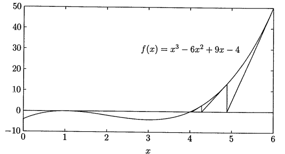
A relação anterior demonstra que a equação não-linear $\small f(x) - c = 0$ é aproximada pela linha tangente à curva no ponto $\small x^{(k)}$. Assim, é obtida uma equação linear em termos de pequenas mudanças na variável.

A interseção da linha tangente no ponto $\small x^{(k)}$ com o eixo $\small x$ resulta em $\small x^{(k + 1)}$. Esta ideia é demonstrada graficamente no exemplo a seguir.

Solução de Equações Algébricas Não-lineares - Método Newton-Raphson - Exemplo 3.3.1

Usar o Método Newton-Raphson, considerando como solução inicial $\small x^{(0)} = 6$, para determinar a raiz da seguinte equação:

$\small f(x) = x^3 - 6x^2 + 9x -4 = 0$

A derivada de $\small f(x)$ é:

$\small \frac{df(x)}{dx} = 3x^2 - 12x + 9$

Na primeira iteração, $\Delta c^{(0)}$ é:

$\small \Delta c^{(0)} = c - f(x^{(0)}) = 0 - 50 = -50$

$\small \left({\frac{df}{dx}}\right)^{(0)} = 45$

$\small \Delta x^{(0)} = \frac{\Delta c^{(0)}}{\left({\frac{df}{dx}}\right)^{(0)}} = \frac{-50}{45} = -1,1111$

Assim, o resultado no final da primeira iteração é:

$\small x^{(1)} = x^{(0)} + \Delta x^{(0)} = 6 - 1,1111 = 4,8889$

Nas iterações subsequentes resultam em:

$\small x^{(2)} = x^{(1)} + \Delta x^{(1)} = 4,8889 - \frac{13,4431}{22,037} = 4,2789$

$\small x^{(3)} = x^{(2)} + \Delta x^{(2)} = 4,2789 - \frac{2,9981}{12,5797} = 4,0405$

$\small x^{(4)} = x^{(3)} + \Delta x^{(3)} = 4,0405 - \frac{0,3748}{9,4914} = 4,0011$

$\small x^{(5)} = x^{(4)} + \Delta x^{(4)} = 4,0011 - \frac{0,0095}{9,0126} = 4,0000$

Pode ser observado que o Método de Newton-Raphson converge consideravelmente mais rapidamente que o Método Gauss-Seidel.

O Método de Newton-Raphson pode convergir a uma raiz diferente da esperada ou então divergir se a aproximação inicial não está o suficientemente próxima da raiz.

Solução de Equações Algébricas Não-lineares - Método Newton-Raphson

Considere agora o seguinte conjunto $\small n$ dimensional de equações:

$\small \begin{array}{*{20}{c}} {{{\left( {{f_1}} \right)}^{(0)}} + {{\left( {\frac{{\partial {f_1}}}{{\partial {x_1}}}} \right)}^{(0)}}\Delta x_1^{(0)} + {{\left( {\frac{{\partial {f_1}}}{{\partial {x_2}}}} \right)}^{(0)}}\Delta x_2^{(0)} + \cdots + {{\left( {\frac{{\partial {f_1}}}{{\partial {x_n}}}} \right)}^{(0)}}\Delta x_n^{(0)} = {c_1}}\\ {{{\left( {{f_2}} \right)}^{(0)}} + {{\left( {\frac{{\partial {f_2}}}{{\partial {x_1}}}} \right)}^{(0)}}\Delta x_1^{(0)} + {{\left( {\frac{{\partial {f_2}}}{{\partial {x_2}}}} \right)}^{(0)}}\Delta x_2^{(0)} + \cdots + {{\left( {\frac{{\partial {f_2}}}{{\partial {x_n}}}} \right)}^{(0)}}\Delta x_n^{(0)} = {c_2}}\\ \vdots \\ {{{\left( {{f_n}} \right)}^{(0)}} + {{\left( {\frac{{\partial {f_n}}}{{\partial {x_1}}}} \right)}^{(0)}}\Delta x_1^{(0)} + {{\left( {\frac{{\partial {f_n}}}{{\partial {x_2}}}} \right)}^{(0)}}\Delta x_2^{(0)} + \cdots + {{\left( {\frac{{\partial {f_n}}}{{\partial {x_n}}}} \right)}^{(0)}}\Delta x_n^{(0)} = {c_n}} \end{array}$

Solução de Equações Algébricas Não-lineares - Método Newton-Raphson

Ou na forma matricial:

$\scriptsize \left[ {\begin{array}{*{20}{c}} {{c_1} - {{\left( {{f_1}} \right)}^{(0)}}}\\ {{c_2} - {{\left( {{f_2}} \right)}^{(0)}}}\\ \vdots \\ {{c_n} - {{\left( {{f_n}} \right)}^{(0)}}} \end{array}} \right] = \left[ {\begin{array}{*{20}{c}} {{{\left( {\frac{{\partial {f_1}}}{{\partial {x_1}}}} \right)}^{(0)}}}&{{{\left( {\frac{{\partial {f_1}}}{{\partial {x_{2}}}}} \right)}^{(0)}}}& \cdots &{{{\left( {\frac{{\partial {f_1}}}{{\partial {x_n}}}} \right)}^{(0)}}}\\ {{{\left( {\frac{{\partial {f_2}}}{{\partial {x_1}}}} \right)}^{(0)}}}&{{{\left( {\frac{{\partial {f_2}}}{{\partial {x_{2}}}}} \right)}^{(0)}}}& \cdots &{{{\left( {\frac{{\partial {f_2}}}{{\partial {x_n}}}} \right)}^{(0)}}}\\ \vdots & \vdots & \ddots & \vdots \\ {{{\left( {\frac{{\partial {f_n}}}{{\partial {x_1}}}} \right)}^{(0)}}}&{{{\left( {\frac{{\partial {f_n}}}{{\partial {x_{2}}}}} \right)}^{(0)}}}& \cdots &{{{\left( {\frac{{\partial {f_n}}}{{\partial {x_n}}}} \right)}^{(0)}}} \end{array}} \right]\left[ {\begin{array}{*{20}{c}} {\Delta x_1^{(0)}}\\ {\Delta x_2^{(0)}}\\ \vdots \\ {\Delta x_n^{(0)}} \end{array}} \right]$

Em forma compacta, pode ser escrito como:

$\small \Delta C^{(k)} = J^{(k)} \Delta X^{(k)}$

$\small \Delta X^{(k)} = \left[{ J^{(k)} }\right] ^{-1} \Delta C^{(k)} $

Solução de Equações Algébricas Não-lineares - Método Newton-Raphson

$\small \Delta X^{(k)} = \left[{ J^{(k)} }\right] ^{-1} \Delta C^{(k)} $

A atualização das variáveis usando o Método de Newton-Raphson, para o sistema $\small n$ dimensional, fica então:

$\small X^{(k + 1)} = X^{(k)} + \Delta X^{(k)} $

Sendo:

$\tiny \Delta {X^{(k)}} = \left[ {\begin{array}{*{20}{c}} {\Delta x_1^{(k)}}\\ {\Delta x_2^{(k)}}\\ \vdots \\ {\Delta x_n^{(k)}} \end{array}} \right];{\rm{ }}\Delta {C^{(k)}} = \left[ {\begin{array}{*{20}{c}} {{c_1} - {{\left( {{f_1}} \right)}^{(k)}}}\\ {{c_2} - {{\left( {{f_2}} \right)}^{(k)}}}\\ \vdots \\ {{c_n} - {{\left( {{f_n}} \right)}^{(k)}}} \end{array}} \right];{\rm{ }}{J^{(k)}} = \left[ {\begin{array}{*{20}{c}} {{{\left( {\frac{{\partial {f_1}}}{{\partial {x_1}}}} \right)}^{(k)}}}&{{{\left( {\frac{{\partial {f_1}}}{{\partial {x_{2}}}}} \right)}^{(k)}}}& \cdots &{{{\left( {\frac{{\partial {f_1}}}{{\partial {x_n}}}} \right)}^{(k)}}}\\ {{{\left( {\frac{{\partial {f_2}}}{{\partial {x_1}}}} \right)}^{(k)}}}&{{{\left( {\frac{{\partial {f_2}}}{{\partial {x_{2}}}}} \right)}^{(k)}}}& \cdots &{{{\left( {\frac{{\partial {f_2}}}{{\partial {x_n}}}} \right)}^{(k)}}}\\ \vdots & \vdots & \ddots & \vdots \\ {{{\left( {\frac{{\partial {f_n}}}{{\partial {x_1}}}} \right)}^{(k)}}}&{{{\left( {\frac{{\partial {f_n}}}{{\partial {x_{2}}}}} \right)}^{(k)}}}& \cdots &{{{\left( {\frac{{\partial {f_n}}}{{\partial {x_n}}}} \right)}^{(k)}}} \end{array}} \right]$

Solução de Equações Algébricas Não-lineares - Método Newton-Raphson

$\small J^{(k)}$ é chamada de Matriz Jacobiana. Os elementos desta matriz são as derivadas parciais avaliadas no ponto $\small X^{(k)}$.

É assumido que $\small J^{(k)}$ tem inversa em cada iteração.

O Método de Newton-Raphson, quando aplicado a um conjunto de equações não-lineares, reduz o problema à resolução de um sistema de equações lineares.

Exemplo de Aplicação do Método Newton-Raphson: Fluxo de Potência

Para um sistema de potência típico, como o apresentado na figura anterior, a corrente injetada na barra $\small i$ é dada por:

$\small I_i = \sum\limits_{j = 1}^{n} {Y_{ij} V_j} $

Exemplo de Aplicação do Método Newton-Raphson: Fluxo de Potência

$\small \begin{array}{*{20}{c}} {I_i = \sum\limits_{j = 1}^{n} {Y_{ij} V_j} ; }&{ i = 1, \cdots, n } \end{array} $

Rescrevendo a anterior equação, considerando que $\small Y_{ij} = G_{ij} + jB_{ij}$, tem-se que:

$\small \begin{array}{*{20}{c}} {I_i = \sum\limits_{j = 1}^{n} { \left({ G_{ij} + jB_{ij} } \right) V_j }; }&{ i = 1, \cdots, n } \end{array} $

Por outro lado, sabe-se que a potência complexa na barra $\small i$ é:

$\small \begin{array}{*{20}{c}} {P_i + jQ_i = V_i I_i^*; }&{ i = 1, \cdots, n } \end{array} $

Exemplo de Aplicação do Método Newton-Raphson: Fluxo de Potência

$\small \begin{array}{*{20}{c}} {P_i + jQ_i = V_i I_i^*; }&{ i = 1, \cdots, n } \end{array} $

Substituindo a expressão de corrente na anterior equação, tem-se que:

$\small \begin{array}{*{20}{c}} {P_i + jQ_i = V_i \sum\limits_{j = 1}^{n} { \left({ G_{ij} - jB_{ij} } \right) V_j^* }; }&{ i = 1, \cdots, n } \end{array} $

ou:

$\small \begin{array}{*{20}{c}} {P_i + jQ_i = | V_i | \angle \theta_i \sum\limits_{j = 1}^{n} { \left({ G_{ij} - jB_{ij} } \right) | V_j | \angle - \theta_i }; }&{ i = 1, \cdots, n } \end{array} $

Exemplo de Aplicação do Método Newton-Raphson: Fluxo de Potência

$\small \begin{array}{*{20}{c}} {P_i + jQ_i = | V_i | \angle \theta_i \sum\limits_{j = 1}^{n} { \left({ G_{ij} - jB_{ij} } \right) | V_j | \angle - \theta_i }; }&{ i = 1, \cdots, n } \end{array} $

Separando a parte real, definindo $\small \theta_{ij} = \theta_i - \theta_j$, tem-se que:

$\small \begin{array}{*{20}{c}} { P_i = {{\mathop{\rm Re}\nolimits} \left\{ {| V_i | \angle \theta_i \sum\limits_{j = 1}^{n} { \left({ G_{ij} - jB_{ij} } \right) | V_j | \angle - \theta_i }} \right\}} ; }&{ i = 1, \cdots, n } \end{array} $

$\small \begin{array}{*{20}{c}} { P_i = {{\mathop{\rm Re}\nolimits} \left\{ {\sum\limits_{j = 1}^{n} { | V_i | \angle \theta_i \left({ G_{ij} - jB_{ij} } \right) | V_j | \angle - \theta_i }} \right\}} ; }&{ i = 1, \cdots, n } \end{array} $

Exemplo de Aplicação do Método Newton-Raphson: Fluxo de Potência

$\small \begin{array}{*{20}{c}} { P_i = {{\mathop{\rm Re}\nolimits} \left\{ {\sum\limits_{j = 1}^{n} { | V_i | | V_j | \angle \left({ \theta_i - \theta_j }\right) \left({ G_{ij} - jB_{ij} } \right) }} \right\}} ; }&{ i = 1, \cdots, n } \end{array} $

$\small \begin{array}{*{20}{c}} { P_i = {{\mathop{\rm Re}\nolimits} \left\{ {\sum\limits_{j = 1}^{n} { | V_i | | V_j | \angle \theta_{ij} \left({ G_{ij} - jB_{ij} } \right) }} \right\}} ; }&{ i = 1, \cdots, n } \end{array} $

$\small \begin{array}{*{20}{c}} { P_i = {{\mathop{\rm Re}\nolimits} \left\{ {\sum\limits_{j = 1}^{n} { | V_i | | V_j | G_{ij} \angle \theta_{ij} - j | V_i | | V_j | B_{ij} \angle \theta_{ij} }} \right\}} ; }&{ i = 1, \cdots, n } \end{array} $

Exemplo de Aplicação do Método Newton-Raphson: Fluxo de Potência

Assim, a injeção de potência ativa, para $\small i = 1, \cdots, n$, é:

$\scriptsize P_i = { { | V_i | \sum\limits_{j = 1}^{n} { \left\{ { | V_j | G_{ij} cos \left({ \theta_{ij} }\right) + | V_j | B_{ij} sen \left({ \theta_{ij} }\right) } \right\} }} } $

Similarmente, separando a parte imaginária, a injeção de potência reativa, para $\small i = 1, \cdots, n$, é:

$\scriptsize Q_i = { { | V_i | \sum\limits_{j = 1}^{n} { \left\{ { | V_j | G_{ij} sen \left({ \theta_{ij} }\right) - | V_j | B_{ij} cos \left({ \theta_{ij} }\right) } \right\} }} } $

Fluxo de Potência - Método Newton-Raphson - Exemplo 3.3.2

Escrever as equações do fluxo de potência para o sistema da figura.

Equações do fluxo de potência:

$\small \begin{array}{*{20}{c}} { P_i = { { | V_i | \sum\limits_{j = 1}^{n} { \left\{ { | V_j | G_{ij} cos \left({ \theta_{ij} }\right) + | V_j | B_{ij} sen \left({ \theta_{ij} }\right) } \right\} }} } ; }&{ i = 1, \cdots, n } \end{array} $

$\small \begin{array}{*{20}{c}} { Q_i = { { | V_i | \sum\limits_{j = 1}^{n} { \left\{ { | V_j | G_{ij} sen \left({ \theta_{ij} }\right) - | V_j | B_{ij} cos \left({ \theta_{ij} }\right) } \right\} }} } ; }&{ i = 1, \cdots, n } \end{array} $

Resolvendo para cada uma das barras do sistema:

$\scriptsize \begin{array}{*{20}{c}} \begin{array}{l} {P_1} = \left| {{V_1}} \right|\left[ {{V_1}\left\{ {{G_{11}}\cos \left( {{\theta _{11}}} \right) + {B_{11}}sen\left( {{\theta _{11}}} \right)} \right\} + } \right.\\ \begin{array}{*{20}{c}} {}&{\left. {{V_2}\left\{ {{G_{12}}\cos \left( {{\theta _{12}}} \right) + {B_{12}}sen\left( {{\theta _{12}}} \right)} \right\} + {V_3}\left\{ {{G_{13}}\cos \left( {{\theta _{13}}} \right) + {B_{13}}sen\left( {{\theta _{13}}} \right)} \right\}} \right]} \end{array} \end{array}\\ \begin{array}{l} {P_2} = \left| {{V_2}} \right|\left[ {{V_1}\left\{ {{G_{21}}\cos \left( {{\theta _{21}}} \right) + {B_{21}}sen\left( {{\theta _{21}}} \right)} \right\} + } \right.\\ \begin{array}{*{20}{c}} {}&{\left. {{V_2}\left\{ {{G_{22}}\cos \left( {{\theta _{22}}} \right) + {B_{22}}sen\left( {{\theta _{22}}} \right)} \right\} + {V_3}\left\{ {{G_{23}}\cos \left( {{\theta _{23}}} \right) + {B_{23}}sen\left( {{\theta _{23}}} \right)} \right\}} \right]} \end{array} \end{array}\\ \begin{array}{l} {P_3} = \left| {{V_3}} \right|\left[ {{V_3}\left\{ {{G_{31}}\cos \left( {{\theta _{31}}} \right) + {B_{31}}sen\left( {{\theta _{31}}} \right)} \right\} + } \right.\\ \begin{array}{*{20}{c}} {}&{\left. {{V_2}\left\{ {{G_{32}}\cos \left( {{\theta _{32}}} \right) + {B_{32}}sen\left( {{\theta _{32}}} \right)} \right\} + {V_3}\left\{ {{G_{33}}\cos \left( {{\theta _{33}}} \right) + {B_{33}}sen\left( {{\theta _{33}}} \right)} \right\}} \right]} \end{array} \end{array} \end{array} $

$\scriptsize \begin{array}{*{20}{c}} \begin{array}{l} {Q_1} = \left| {{V_1}} \right|\left[ {{V_1}\left\{ {{G_{11}}sen\left( {{\theta _{11}}} \right) - {B_{11}}\cos \left( {{\theta _{11}}} \right)} \right\} + } \right.\\ \begin{array}{*{20}{c}} {}&{\left. {{V_2}\left\{ {{G_{12}}\cos \left( {{\theta _{12}}} \right) - {B_{12}}\cos \left( {{\theta _{12}}} \right)} \right\} + {V_3}\left\{ {{G_{13}}sen\left( {{\theta _{13}}} \right) - {B_{13}}\cos \left( {{\theta _{13}}} \right)} \right\}} \right]} \end{array} \end{array}\\ \begin{array}{l} {Q_2} = \left| {{V_2}} \right|\left[ {{V_1}\left\{ {{G_{21}}sen\left( {{\theta _{21}}} \right) - {B_{21}}\cos \left( {{\theta _{21}}} \right)} \right\} + } \right.\\ \begin{array}{*{20}{c}} {}&{\left. {{V_2}\left\{ {{G_{22}}\cos \left( {{\theta _{22}}} \right) - {B_{22}}\cos \left( {{\theta _{22}}} \right)} \right\} + {V_3}\left\{ {{G_{23}}sen\left( {{\theta _{23}}} \right) - {B_{23}}\cos \left( {{\theta _{23}}} \right)} \right\}} \right]} \end{array} \end{array}\\ \begin{array}{l} {Q_3} = \left| {{V_3}} \right|\left[ {{V_3}\left\{ {{G_{31}}sen\left( {{\theta _{31}}} \right) - {B_{31}}\cos \left( {{\theta _{31}}} \right)} \right\} + } \right.\\ \begin{array}{*{20}{c}} {}&{\left. {{V_2}\left\{ {{G_{32}}sen\left( {{\theta _{32}}} \right) - {B_{32}}\cos \left( {{\theta _{32}}} \right)} \right\} + {V_3}\left\{ {{G_{33}}sen\left( {{\theta _{33}}} \right) - {B_{33}}\cos \left( {{\theta _{33}}} \right)} \right\}} \right]} \end{array} \end{array} \end{array}$

Exemplo de Aplicação do Método Newton-Raphson: Fluxo de Potência

Devido à variedade de tipos de barra, o sistema de equações que descreve o sistema elétrico é dividido em dois subsistemas:

Subsistema 1: Este subsistema contém as equações que devem ser resolvidas para se encontrar a solução do fluxo de potência, ou seja, módulo e ângulo das tensões nas barras:

$\small P_i = P_i (|V|, \theta)$; $\small i \in \{ PQ, PV \}$ $\small \rightarrow$ Barras de carga e de tensão controlada.
$\small Q_i = Q_i (|V|, \theta)$; $\small i \in \{ PQ \}$ $\small \rightarrow$ Barras de carga.

Subsistema 2: As incógnitas aqui contidas são determinadas por substituição das variáveis calculadas no Subsistema 1:

$\small P_i = P_i (|V|, \theta)$; $\small i \in \{ V \theta \}$ $\small \rightarrow$ Barra de folga.
$\small Q_i = Q_i (|V|, \theta)$; $\small i \in \{ V \theta, PV \}$ $\small \rightarrow$ Barra de folga e barras de tensão controlada.

Fluxo de Potência - Método Newton-Raphson - Exemplo 3.3.3

Escrever as equações do sistema da figura, separando-as nos subsistemas 1 e 2.

Equações do fluxo de potência para o Subsistema 1 ($\small P$ para barras tipo $\small PQ$ e $\small PV$, e $\small Q$ para barras tipo $\small PQ$) :

$\scriptsize \begin{array}{*{20}{c}} \begin{array}{l} {P_2} = \left| {{V_2}} \right|\left[ {{V_1}\left\{ {{G_{21}}\cos \left( {{\theta _{21}}} \right) + {B_{21}}sen\left( {{\theta _{21}}} \right)} \right\} + } \right.\\ \begin{array}{*{20}{c}} {}&{\left. {{V_2}\left\{ {{G_{22}}\cos \left( {{\theta _{22}}} \right) + {B_{22}}sen\left( {{\theta _{22}}} \right)} \right\} + {V_3}\left\{ {{G_{23}}\cos \left( {{\theta _{23}}} \right) + {B_{23}}sen\left( {{\theta _{23}}} \right)} \right\}} \right]} \end{array} \end{array}\\ \begin{array}{l} {P_3} = \left| {{V_3}} \right|\left[ {{V_3}\left\{ {{G_{31}}\cos \left( {{\theta _{31}}} \right) + {B_{31}}sen\left( {{\theta _{31}}} \right)} \right\} + } \right.\\ \begin{array}{*{20}{c}} {}&{\left. {{V_2}\left\{ {{G_{32}}\cos \left( {{\theta _{32}}} \right) + {B_{32}}sen\left( {{\theta _{32}}} \right)} \right\} + {V_3}\left\{ {{G_{33}}\cos \left( {{\theta _{33}}} \right) + {B_{33}}sen\left( {{\theta _{33}}} \right)} \right\}} \right]} \end{array} \end{array} \\ \begin{array}{l} {Q_3} = \left| {{V_3}} \right|\left[ {{V_3}\left\{ {{G_{31}}sen\left( {{\theta _{31}}} \right) - {B_{31}}\cos \left( {{\theta _{31}}} \right)} \right\} + } \right.\\ \begin{array}{*{20}{c}} {}&{\left. {{V_2}\left\{ {{G_{32}}sen\left( {{\theta _{32}}} \right) - {B_{32}}\cos \left( {{\theta _{32}}} \right)} \right\} + {V_3}\left\{ {{G_{33}}sen\left( {{\theta _{33}}} \right) - {B_{33}}\cos \left( {{\theta _{33}}} \right)} \right\}} \right]} \end{array} \end{array} \end{array} $

A solução das três equações acima fornece $\small V_3$, $\small \theta_2$, $\small \theta_3$.

Equações do flxo de potência para o Subsistema 2 ($\small P$ para a barra tipo $\small V \theta$, e $\small Q$ para a barra tipo $\small V \theta$ e as barras tipo $\small PV$):

$\scriptsize \begin{array}{*{20}{c}} \begin{array}{l} {P_1} = \left| {{V_1}} \right|\left[ {{V_1}\left\{ {{G_{11}}\cos \left( {{\theta _{11}}} \right) + {B_{11}}sen\left( {{\theta _{11}}} \right)} \right\} + } \right.\\ \begin{array}{*{20}{c}} {}&{\left. {{V_2}\left\{ {{G_{12}}\cos \left( {{\theta _{12}}} \right) + {B_{12}}sen\left( {{\theta _{12}}} \right)} \right\} + {V_3}\left\{ {{G_{13}}\cos \left( {{\theta _{13}}} \right) + {B_{13}}sen\left( {{\theta _{13}}} \right)} \right\}} \right]} \end{array} \end{array}\\ \begin{array}{l} {Q_1} = \left| {{V_1}} \right|\left[ {{V_1}\left\{ {{G_{11}}sen\left( {{\theta _{11}}} \right) - {B_{11}}\cos \left( {{\theta _{11}}} \right)} \right\} + } \right.\\ \begin{array}{*{20}{c}} {}&{\left. {{V_2}\left\{ {{G_{12}}\cos \left( {{\theta _{12}}} \right) - {B_{12}}\cos \left( {{\theta _{12}}} \right)} \right\} + {V_3}\left\{ {{G_{13}}sen\left( {{\theta _{13}}} \right) - {B_{13}}\cos \left( {{\theta _{13}}} \right)} \right\}} \right]} \end{array} \end{array}\\ \begin{array}{l} {Q_3} = \left| {{V_3}} \right|\left[ {{V_3}\left\{ {{G_{31}}sen\left( {{\theta _{31}}} \right) - {B_{31}}\cos \left( {{\theta _{31}}} \right)} \right\} + } \right.\\ \begin{array}{*{20}{c}} {}&{\left. {{V_2}\left\{ {{G_{32}}sen\left( {{\theta _{32}}} \right) - {B_{32}}\cos \left( {{\theta _{32}}} \right)} \right\} + {V_3}\left\{ {{G_{33}}sen\left( {{\theta _{33}}} \right) - {B_{33}}\cos \left( {{\theta _{33}}} \right)} \right\}} \right]} \end{array} \end{array} \end{array} $

Para determinar as outras variáveis, do Subsistema 2, basta substituir as variáveis calculadas no Subsistema 1 nas equações acima.

Exemplo de Aplicação do Método Newton-Raphson: Fluxo de Potência

Definindo os "resíduos de potência" como:

$\small \begin{array}{*{20}{c}} { \Delta P_i = P_i^{esp} - P_i^{cal} (|V|, \theta); }&{ i \in \{ PQ, PV \} } \end{array} $

$\small \begin{array}{*{20}{c}} { \Delta Q_i = Q_i^{esp} - Q_i^{cal} (|V|, \theta); }&{ i \in \{ PQ \} } \end{array} $

o sistema a ser resolvido pelo Método de Newton-Raphson é:

$\small \begin{array}{*{20}{c}} { \Delta P = 0; }&{ i \in \{ PQ, PV \} } \end{array} $

$\small \begin{array}{*{20}{c}} { \Delta Q = 0; }&{ i \in \{ PQ \} } \end{array} $

Considera-se então o sistema com $\small n$ barras, sendo que:

Barras $\small PQ$: barras de 1 até $\small l$ ($\small n_{PQ} = l$).
Barras $\small PV$: barras de $\small l$ + 1 até $\small n$ - 1 ($\small n_{PV} = n - l - 1$).
Barras $\small V \theta$: barra $\small n$ ($\small n_{V \theta} = 1$).

Exemplo de Aplicação do Método Newton-Raphson: Fluxo de Potência

Relembrando, do Método de Newton-Raphson, na forma geral, tem-se que:

$\small \Delta X^{(k)} = \left[{ J^{(k)} }\right] ^{-1} \Delta C^{(k)} $

A atualização das variáveis usando o Método de Newton-Raphson, para o sistema $\small n$ dimensional, é:

$\small X^{(k + 1)} = X^{(k)} + \Delta X^{(k)} $

Sendo:

$\tiny \Delta {X^{(k)}} = \left[ {\begin{array}{*{20}{c}} {\Delta x_1^{(k)}}\\ {\Delta x_2^{(k)}}\\ \vdots \\ {\Delta x_n^{(k)}} \end{array}} \right];{\rm{ }}\Delta {C^{(k)}} = \left[ {\begin{array}{*{20}{c}} {{c_1} - {{\left( {{f_1}} \right)}^{(k)}}}\\ {{c_2} - {{\left( {{f_2}} \right)}^{(k)}}}\\ \vdots \\ {{c_n} - {{\left( {{f_n}} \right)}^{(k)}}} \end{array}} \right];{\rm{ }}{J^{(k)}} = \left[ {\begin{array}{*{20}{c}} {{{\left( {\frac{{\partial {f_1}}}{{\partial {x_1}}}} \right)}^{(k)}}}&{{{\left( {\frac{{\partial {f_1}}}{{\partial {x_{`2}}}}} \right)}^{(k)}}}& \cdots &{{{\left( {\frac{{\partial {f_1}}}{{\partial {x_n}}}} \right)}^{(k)}}}\\ {{{\left( {\frac{{\partial {f_2}}}{{\partial {x_1}}}} \right)}^{(k)}}}&{{{\left( {\frac{{\partial {f_2}}}{{\partial {x_{`2}}}}} \right)}^{(k)}}}& \cdots &{{{\left( {\frac{{\partial {f_2}}}{{\partial {x_n}}}} \right)}^{(k)}}}\\ \vdots & \vdots & \ddots & \vdots \\ {{{\left( {\frac{{\partial {f_n}}}{{\partial {x_1}}}} \right)}^{(k)}}}&{{{\left( {\frac{{\partial {f_n}}}{{\partial {x_{`2}}}}} \right)}^{(k)}}}& \cdots &{{{\left( {\frac{{\partial {f_n}}}{{\partial {x_n}}}} \right)}^{(k)}}} \end{array}} \right]$

Fluxo de Potência - Método Newton-Raphson

Nas expressões:

$\small \Delta X^{(k)} = \left[{ J^{(k)} }\right] ^{-1} \Delta C^{(k)} $

$\small X^{(k + 1)} = X^{(k)} + \Delta X^{(k)} $

Podem-se usar, para o Subsistema 1, as seguintes relações:

$\scriptsize \Delta C^{(k)} = {\left[ {\begin{array}{*{20}{c}} {\Delta {P_1}}&{\Delta {P_2}}& \cdots &{\Delta {P_l}}&{\Delta {P_{l + 1}}}& \cdots &{\Delta {P_{n - 1}}}&{\Delta {Q_1}}&{\Delta {Q_2}}& \cdots &{\Delta {Q_l}} \end{array}} \right]^T} $

$\scriptsize X^{(k)} = {\left[ {\begin{array}{*{20}{c}} {{\theta _1}}&{{\theta _2}}& \cdots &{{\theta _l}}&{{\theta _{l + 1}}}& \cdots &{{\theta _{n - 1}}}&{{V_1}}&{{V_2}}& \cdots &{{V_l}} \end{array}} \right]^T} $

$\scriptsize \Delta X^{(k)} = {\left[ {\begin{array}{*{20}{c}} {{\Delta \theta _1}}&{{\Delta \theta _2}}& \cdots &{{\Delta \theta _l}}&{{\Delta \theta _{l + 1}}}& \cdots &{{\Delta \theta _{n - 1}}}&{{\Delta V_1}}&{{\Delta V_2}}& \cdots &{{\Delta V_l}} \end{array}} \right]^T} $

Exemplo de Aplicação do Método Newton-Raphson: Fluxo de Potência

Ou:

$\scriptsize \Delta C^{(k)} = {\left[ {\begin{array}{*{20}{c}} {\underline {\Delta P} }\\ {\underline {\Delta Q} } \end{array}} \right]^{(k)}} $

$\scriptsize X^{(k)} = {\left[ {\begin{array}{*{20}{c}} {\underline \theta }\\ {\underline V } \end{array}} \right]^{(k)}} $

$\scriptsize \Delta X^{(k)} = {\left[ {\begin{array}{*{20}{c}} {\underline {\Delta \theta} }\\ {\underline {\Delta V} } \end{array}} \right]^{(k)}} $

Exemplo de Aplicação do Método Newton-Raphson: Fluxo de Potência

$\scriptsize \Delta C^{(k)} = {\left[ {\begin{array}{*{20}{c}} {\underline {\Delta P} }\\ {\underline {\Delta Q} } \end{array}} \right]^{(k)}} $

$\scriptsize X^{(k)} = {\left[ {\begin{array}{*{20}{c}} {\underline \theta }\\ {\underline V } \end{array}} \right]^{(k)}} $

$\scriptsize \Delta X^{(k)} = {\left[ {\begin{array}{*{20}{c}} {\underline {\Delta \theta} }\\ {\underline {\Delta V} } \end{array}} \right]^{(k)}} $

Assim, tem-se que:

$\small \Delta X^{(k)} = \left[{ J^{(k)} }\right] ^{-1} \Delta C^{(k)} $

$\small {\left[ {\begin{array}{*{20}{c}} {\underline {\Delta \theta } }\\ {\underline {\Delta V} } \end{array}} \right]^{(k)}} = \left[{ J^{(k)} }\right] ^{-1} {\left[ {\begin{array}{*{20}{c}} {\underline {\Delta P} }\\ {\underline {\Delta Q} } \end{array}} \right]^{(k)}} $

Exemplo de Aplicação do Método Newton-Raphson: Fluxo de Potência

A atualização das variáveis, na solução do Subsistema 1, é então:

$\small {\left[ {\begin{array}{*{20}{c}} {\underline \theta }\\ {\underline V } \end{array}} \right]^{(k + 1)}} = {\left[ {\begin{array}{*{20}{c}} {\underline \theta }\\ {\underline V } \end{array}} \right]^{(k)}} + {\left[ {\begin{array}{*{20}{c}} {\underline {\Delta \theta } }\\ {\underline {\Delta V} } \end{array}} \right]^{(k)}} $

A convergência é conferida de acordo com:

$\small \left\{ {\left| {\underline {\Delta P} } \right|} \right\} \le {\varepsilon _P} $

$\small \left\{ {\left| {\underline {\Delta Q} } \right|} \right\} \le {\varepsilon _Q} $

Exemplo de Aplicação do Método Newton-Raphson: Fluxo de Potência

$\small {\left[ {\begin{array}{*{20}{c}} {\underline {\Delta P} }\\ {\underline {\Delta Q} } \end{array}} \right]^{(k)}} = \left[{ J^{(k)} }\right] {\left[ {\begin{array}{*{20}{c}} {\underline {\Delta \theta } }\\ {\underline {\Delta V} } \end{array}} \right]^{(k)}} $

Decompondo a matriz Jacobiana (lembrando que $\small n_{PQ} = l$ e $\small n_{PV} = n - l - 1$):

$\small {J_{(n + l - 1)(n + l - 1)}} = \left[ {\begin{array}{*{20}{c}} {{{\partial \underline {\Delta P} }}/{{\partial \underline \theta }}}&{{{\partial \underline {\Delta P} }}/{{\partial \underline V }}}\\ {{{\partial \underline {\Delta Q} }}/{{\partial \underline \theta }}}&{{{\partial \underline {\Delta Q} }}/{{\partial \underline V }}} \end{array}} \right] $

Exemplo de Aplicação do Método Newton-Raphson: Fluxo de Potência

$\scriptsize {J_{(n + l - 1)(n + l - 1)}} = \left[ {\begin{array}{*{20}{c}} {{{\partial \underline {\Delta P} }}/{{\partial \underline \theta }}}&{{{\partial \underline {\Delta P} }}/{{\partial \underline V }}}\\ {{{\partial \underline {\Delta Q} }}/{{\partial \underline \theta }}}&{{{\partial \underline {\Delta Q} }}/{{\partial \underline V }}} \end{array}} \right] $

Lembrando que:

$\scriptsize \Delta P_i = P_i^{esp} - P_i^{cal} (|V|, \theta) = P_i^{esp} - P_i^{cal} $

$\scriptsize \Delta Q_i = Q_i^{esp} - Q_i^{cal} (|V|, \theta) = Q_i^{esp} - Q_i^{cal} $

então:

$\small \begin{array}{*{20}{c}} { \frac{{\partial {\Delta P_i} }}{{\partial \ \theta_j }} = \frac{{\partial \left( {\underline {{P_i^{esp}}} - \underline {{P_i^{cal}}} } \right)}}{{\partial \theta_j }} = \frac{{\partial { {P_i^{cal}}} }}{{\partial \theta_j }} = \frac{{\partial { P_i} }}{{\partial \theta_j }} ;}&{ \frac{{\partial {\Delta P_i} }}{{\partial \ V_j }} = \frac{{\partial \left( {\underline {{P_i^{esp}}} - \underline {{P_i^{cal}}} } \right)}}{{\partial V_j }} = \frac{{\partial { {P_i^{cal}}} }}{{\partial V_j }} = \frac{{\partial { P_i} }}{{\partial V_j }} }\\ { \frac{{\partial {\Delta Q_i} }}{{\partial \ \theta_j }} = \frac{{\partial \left( {\underline {{Q_i^{esp}}} - \underline {{Q_i^{cal}}} } \right)}}{{\partial \theta_j }} = \frac{{\partial { {Q_i^{cal}}} }}{{\partial \theta_j }} = \frac{{\partial { Q_i} }}{{\partial \theta_j }} ;}&{ \frac{{\partial {\Delta Q_i} }}{{\partial \ V_j }} = \frac{{\partial \left( {\underline {{Q_i^{esp}}} - \underline {{Q_i^{cal}}} } \right)}}{{\partial V_j }} = \frac{{\partial { {Q_i^{cal}}} }}{{\partial V_j }} = \frac{{\partial { Q_i} }}{{\partial V_j }} } \end{array} $

Exemplo de Aplicação do Método Newton-Raphson: Fluxo de Potência

Assim, tem-se que:

ou:

$\small {J_{(n + l - 1)(n + l - 1)}} = \left[ {\begin{array}{*{20}{c}} {{{\partial \underline { P} }}/{{\partial \underline \theta }}}&{{{\partial \underline { P} }}/{{\partial \underline V }}}\\ {{{\partial \underline { Q} }}/{{\partial \underline \theta }}}&{{{\partial \underline { Q} }}/{{\partial \underline V }}} \end{array}} \right] $

Exemplo de Aplicação do Método Newton-Raphson: Fluxo de Potência

Expandindo a matriz Jacobiana, tem-se que:

$\scriptsize \begin{array}{l} {J_{(n - 1 + l)(n - 1 + l)}} = \left[ {\begin{array}{*{20}{c}} {\frac{{\partial {P_1}}}{{\partial {\theta _1}}}}&{\frac{{\partial {P_1}}}{{\partial {\theta _2}}}}& \cdots &{\frac{{\partial {P_1}}}{{\partial {\theta _{n - 1}}}}}&|&{\frac{{\partial {P_1}}}{{\partial {V_1}}}}&{\frac{{\partial {P_1}}}{{\partial {V_2}}}}& \cdots &{\frac{{\partial {P_1}}}{{\partial {V_l}}}}\\ {\frac{{\partial {P_2}}}{{\partial {\theta _1}}}}&{\frac{{\partial {P_2}}}{{\partial {\theta _2}}}}& \cdots &{\frac{{\partial {P_2}}}{{\partial {\theta _{n - 1}}}}}&|&{\frac{{\partial {P_2}}}{{\partial {V_1}}}}&{\frac{{\partial {P_2}}}{{\partial {V_2}}}}& \cdots &{\frac{{\partial {P_2}}}{{\partial {V_l}}}}\\ \vdots & \vdots &H& \vdots &|& \vdots & \vdots &N& \vdots \\ {\frac{{\partial {P_{n - 1}}}}{{\partial {\theta _1}}}}&{\frac{{\partial {P_{n - 1}}}}{{\partial {\theta _2}}}}& \cdots &{\frac{{\partial {P_{n - 1}}}}{{\partial {\theta _{n - 1}}}}}&|&{\frac{{\partial {P_{n - 1}}}}{{\partial {V_1}}}}&{\frac{{\partial {P_{n - 1}}}}{{\partial {V_2}}}}& \cdots &{\frac{{\partial {P_{n - 1}}}}{{\partial {V_l}}}}\\ {--}&{--}&{--}&{--}&|&{--}&{--}&{--}&{--}\\ {\frac{{\partial {Q_1}}}{{\partial {\theta _1}}}}&{\frac{{\partial {Q_1}}}{{\partial {\theta _2}}}}& \cdots &{\frac{{\partial {Q_1}}}{{\partial {\theta _{n - 1}}}}}&|&{\frac{{\partial {Q_1}}}{{\partial {V_1}}}}&{\frac{{\partial {Q_1}}}{{\partial {V_2}}}}& \cdots &{\frac{{\partial {Q_1}}}{{\partial {V_l}}}}\\ {\frac{{\partial {Q_2}}}{{\partial {\theta _1}}}}&{\frac{{\partial {Q_2}}}{{\partial {\theta _2}}}}& \cdots &{\frac{{\partial {Q_2}}}{{\partial {\theta _{n - 1}}}}}&|&{\frac{{\partial {Q_2}}}{{\partial {V_1}}}}&{\frac{{\partial {Q_2}}}{{\partial {V_2}}}}& \cdots &{\frac{{\partial {Q_2}}}{{\partial {V_l}}}}\\ \vdots & \vdots &M& \vdots &|& \vdots & \vdots &L& \vdots \\ {\frac{{\partial {Q_l}}}{{\partial {\theta _1}}}}&{\frac{{\partial {Q_l}}}{{\partial {\theta _2}}}}& \cdots &{\frac{{\partial {Q_l}}}{{\partial {\theta _{n - 1}}}}}&|&{\frac{{\partial {Q_l}}}{{\partial {V_1}}}}&{\frac{{\partial {Q_l}}}{{\partial {V_2}}}}& \cdots &{\frac{{\partial {Q_l}}}{{\partial {V_l}}}} \end{array}} \right] \end{array} $

Exemplo de Aplicação do Método Newton-Raphson: Fluxo de Potência

$\small {J_{(n + l - 1)(n + l - 1)}} = \left[ {\begin{array}{*{20}{c}} {H}&{N}\\ {M}&{L} \end{array}} \right] $

$\small {H_{(n - 1)(n - 1)}} = \partial \underline P /\partial \underline \theta $

$\small {N_{(n - 1)(l)}} = \partial \underline P /\partial \underline V $

$\small {M_{(n - 1)(n - 1)}} = \partial \underline Q /\partial \underline \theta $

$\small {L_{(n - 1)(l)}} = \partial \underline Q /\partial \underline V $

Exemplo de Aplicação do Método Newton-Raphson: Fluxo de Potência

Elementos da matriz $\small H$:

$\small \left\{ \begin{array}{l} {H_{ii}} = \frac{\partial P_i}{\partial \theta_i} = - {B_{ii}}V_i^2 - {V_i}\sum\limits_{j \in {\Omega _i}} {{V_j}\left( {{G_{ij}} sen{\theta _{ij}} - {B_{ij}} cos {\theta _{ij}}} \right)} \\ \begin{array}{*{20}{c}} {}& = \end{array} - {B_{ii}}V_i^2 - {Q_i}\\ {H_{ij}} = \frac{\partial P_i}{\partial \theta_j} = {V_i}{V_j}\left( {{G_{ij}} sen{\theta _{ij}} - {B_{ij}} cos {\theta _{ij}}} \right)\\ {H_{ji}} = \frac{\partial P_j}{\partial \theta_i} = - {V_i}{V_j}\left( {{G_{ij}} sen{\theta _{ij}} + {B_{ij}} cos {\theta _{ij}}} \right) \end{array} \right. $

$\small \Omega _i$: Barras conectadas à barra $\small i$, excluindo a própria barra $\small i$.

Exemplo de Aplicação do Método Newton-Raphson: Fluxo de Potência

Elementos da matriz $\small N$:

$\small \left\{ \begin{array}{l} {N_{ii}} = \frac{\partial P_i}{\partial V_i} = {G_{ii}}V_i + \sum\limits_{j \in {\Omega _i}} {{V_j}\left( {{G_{ij}} cos{\theta _{ij}} + {B_{ij}} sen {\theta _{ij}}} \right)} \\ \begin{array}{*{20}{c}} {}& = \end{array} V_i^{-1} \left({ P_i + G_{ii}V_i^2 }\right)\\ {N_{ij}} = \frac{\partial P_i}{\partial V_j} = {V_i}\left( {{G_{ij}} cos{\theta _{ij}} + {B_{ij}} sen {\theta _{ij}}} \right)\\ {N_{ji}} = \frac{\partial P_j}{\partial V_i} = {V_j}\left( {{G_{ij}} cos{\theta _{ij}} - {B_{ij}} sen {\theta _{ij}}} \right) \end{array} \right. $

$\small \Omega _i$: Barras conectadas à barra $\small i$, excluindo a própria barra $\small i$.

Exemplo de Aplicação do Método Newton-Raphson: Fluxo de Potência

Elementos da matriz $\small M$:

$\small \left\{ \begin{array}{l} {M_{ii}} = \frac{\partial Q_i}{\partial \theta_i} = - {G_{ii}}V_i^2 + {V_i}\sum\limits_{j \in {\Omega _i}} {{V_j}\left( {{G_{ij}} cos{\theta _{ij}} + {B_{ij}} sen {\theta _{ij}}} \right)} \\ \begin{array}{*{20}{c}} {}& = \end{array} - {G_{ii}}V_i^2 + {P_i}\\ {M_{ij}} = \frac{\partial Q_i}{\partial \theta_j} = - {V_i}{V_j}\left( {{G_{ij}} cos{\theta _{ij}} + {B_{ij}} sen {\theta _{ij}}} \right)\\ {M_{ji}} = \frac{\partial Q_j}{\partial \theta_i} = - {V_i}{V_j}\left( {{G_{ij}} cos{\theta _{ij}} - {B_{ij}} sen {\theta _{ij}}} \right) \end{array} \right. $

$\small \Omega _i$: Barras conectadas à barra $\small i$, excluindo a própria barra $\small i$.

Exemplo de Aplicação do Método Newton-Raphson: Fluxo de Potência

Elementos da matriz $\small L$:

$\small \left\{ \begin{array}{l} {L_{ii}} = \frac{\partial Q_i}{\partial V_i} = - {B_{ii}}V_i + \sum\limits_{j \in {\Omega _i}} {{V_j}\left( {{G_{ij}} sen{\theta _{ij}} - {B_{ij}} cos {\theta _{ij}}} \right)} \\ \begin{array}{*{20}{c}} {}& = \end{array} V_i^{-1} \left({ Q_i - B_{ii}V_i^2 }\right)\\ {L_{ij}} = \frac{\partial Q_i}{\partial V_j} = {V_i}\left( {{G_{ij}} sen{\theta _{ij}} - {B_{ij}} cos {\theta _{ij}}} \right)\\ {L_{ji}} = \frac{\partial Q_j}{\partial V_i} = - {V_j}\left( {{G_{ij}} sen{\theta _{ij}} + {B_{ij}} cos {\theta _{ij}}} \right) \end{array} \right. $

$\small \Omega _i$: Barras conectadas à barra $\small i$, excluindo a própria barra $\small i$.

Exemplo de Aplicação do Método Newton-Raphson: Fluxo de Potência

Resumo do equacionamento:

$\scriptsize P_i = { { | V_i | \sum\limits_{j = 1}^{n} { \left\{ { | V_j | G_{ij} cos \left({ \theta_{ij} }\right) + | V_j | B_{ij} sen \left({ \theta_{ij} }\right) } \right\} }} } $

$\scriptsize Q_i = { { | V_i | \sum\limits_{j = 1}^{n} { \left\{ { | V_j | G_{ij} sen \left({ \theta_{ij} }\right) - | V_j | B_{ij} cos \left({ \theta_{ij} }\right) } \right\} }} } $

$\tiny {\left[ {\begin{array}{*{20}{c}} {\underline {\Delta P} }\\ {\underline {\Delta Q} } \end{array}} \right]^{(k)}} = \left[ {\begin{array}{*{20}{c}} {H}&{N}\\ {M}&{L} \end{array}} \right] ^{(k)} {\left[ {\begin{array}{*{20}{c}} {\underline {\Delta \theta } }\\ {\underline {\Delta V} } \end{array}} \right]^{(k)}} $

$\tiny {\left[ {\begin{array}{*{20}{c}} {\underline { \theta } }\\ {\underline { V} } \end{array}} \right]^{(k + 1)}} = {\left[ {\begin{array}{*{20}{c}} {\underline { \theta } }\\ {\underline { V} } \end{array}} \right]^{(k)}} + {\left[ {\begin{array}{*{20}{c}} {\underline {\Delta \theta } }\\ {\underline {\Delta V} } \end{array}} \right]^{(k)}} $

Exemplo de Aplicação do Método Newton-Raphson: Fluxo de Potência

Algoritmo do Método Newton-Raphson:

Passo 1: Construir a matriz $\small Y_{\rm{Barra}}$.

Passo 2: Arbitrar valores iniciais das variáveis de estado $\small \underline { \theta}$ para as barras tipo $\small PQ$ e $\small PV$, e $\small \underline { V}$ para as barras tipo $\small PQ$.

Passo 3: Calcular $\small \Delta P_i$ e $\small \Delta Q_i$, de acordo com as seguintes expressões:

$\small \begin{array}{*{20}{c}} { \Delta P_i = P_i^{esp} - P_i^{cal}; }&{ i \in \{ PQ, PV \} } \end{array} $

$\small \begin{array}{*{20}{c}} { \Delta Q_i = Q_i^{esp} - Q_i^{cal}; }&{ i \in \{ PQ \} } \end{array} $

Exemplo de Aplicação do Método Newton-Raphson: Fluxo de Potência

Algoritmo do Método Newton-Raphson:

$\small \begin{array}{*{20}{c}} { \Delta P_i = P_i^{esp} - P_i^{cal} (|V|, \theta); }&{ i \in \{ PQ, PV \} } \end{array} $

$\small \begin{array}{*{20}{c}} { \Delta Q_i = Q_i^{esp} - Q_i^{cal} (|V|, \theta); }&{ i \in \{ PQ \} } \end{array} $

Se:

$\small \left\{ {\left| {\underline {\Delta P} } \right|} \right\} \le {\varepsilon _P} $
$\small \left\{ {\left| {\underline {\Delta Q} } \right|} \right\} \le {\varepsilon _Q} $

então parar; caso contrário, ir ao Passo 4.

Exemplo de Aplicação do Método Newton-Raphson: Fluxo de Potência

Algoritmo do Método Newton-Raphson:

Passo 4: Fazer $\small k = k + 1$. Montar a matriz Jacobiana $\small J^{(k)}$.

Passo 5: Solucionar o sistema linearizado:

$\small {\left[ {\begin{array}{*{20}{c}} {\underline {\Delta P} }\\ {\underline {\Delta Q} } \end{array}} \right]^{(k)}} = J ^{(k)} {\left[ {\begin{array}{*{20}{c}} {\underline {\Delta \theta } }\\ {\underline {\Delta V} } \end{array}} \right]^{(k)}} $

Passo 6: Atualizar a solução do problema:

$\small {\left[ {\begin{array}{*{20}{c}} {\underline { \theta } }\\ {\underline { V} } \end{array}} \right]^{(k + 1)}} = {\left[ {\begin{array}{*{20}{c}} {\underline { \theta } }\\ {\underline { V} } \end{array}} \right]^{(k)}} + {\left[ {\begin{array}{*{20}{c}} {\underline {\Delta \theta } }\\ {\underline {\Delta V} } \end{array}} \right]^{(k)}} $

Passo 7: Voltar ao Passo 3.

Fluxo de Potência - Método Newton-Raphson - Exemplo 3.3.4

Usar o Método Newton-Raphson, considerando como solução inicial $\small \theta_2^{(0)} = 0$ e tolerância em $\small \Delta P = \epsilon = 0,003$, para para resolver o problema de fluxo de potência do sistema elétrico da figura a seguir (dados em pu):

Dados das barras:

Dados da linha:

Montagem da matriz $\small Y_{\rm{Barra}}$:

$\small Y_{12} = \frac{1}{0,0 + j1,0} = 0,19 - j0,96$

$\small Y_{\rm{Barra}} = \left[ {\begin{array}{*{20}{c}} {0,19 - j0,94}&{ - 0,19 + j0,96}\\ { - 0,19 + j0,96}&{0,19 - j0,94} \end{array}} \right]$

Dados das barras:

$\small Y_{\rm{Barra}} = \left[ {\begin{array}{*{20}{c}} {0,19 - j0,94}&{ - 0,19 + j0,96}\\ { - 0,19 + j0,96}&{0,19 - j0,94} \end{array}} \right]$

$\small Y_{\rm{Barra}} = G_{\rm{Barra}} + jB_{\rm{Barra}}$

$\small G_{\rm{Barra}} = \left[ {\begin{array}{*{20}{c}} {0,19 }&{ - 0,19 }\\ { - 0,19 }&{0,19 } \end{array}} \right]$

$\small B_{\rm{Barra}} = \left[ {\begin{array}{*{20}{c}} { - j0,94}&{ j0,96}\\ { j0,96}&{9 - j0,94} \end{array}} \right]$

Solução do Subsistema 1 (não há barras tipo $\small PQ$; portanto, limita-se à solução de $\small \theta$ para a barra tipo $PV$):

Teste de convergência:

$\small P_i = { { | V_i | \sum\limits_{j = 1}^{n} { \left\{ { | V_j | G_{ij} cos \left({ \theta_{ij} }\right) + | V_j | B_{ij} sen \left({ \theta_{ij} }\right) } \right\} }} }$

$\small P_2 = | V_2 | \left\{ { | V_1 | G_{21} cos \left({ \theta_{21} }\right) + | V_1 | B_{21} sen \left({ \theta_{21} }\right) } \right\} + $
$\small | V_2 | \left\{ { | V_2 | G_{22} cos \left({ \theta_{22} }\right) + | V_2 | B_{22} sen \left({ \theta_{22} }\right) } \right\} $

$\small P_2^{(0)} = 0,00$

$\small \Delta P_2^{(0)} = P_2^{esp} - P_2^{cal,(0)} = -0,4 - P_2^{(0)} = - 0,40$

$\small | \Delta P_2^{(0)} | > \epsilon$ $\leftarrow$ Não convergiu.

Processo iterativo pelo Método Newton-Raphson:

Primeira iteração $\small k = 1$:

$\small \Delta P_2^{(1)} = -J^{(1)} \Delta \theta_2^{(1)} $

$\small \Delta P_2^{(1)} = H^{(1)} \Delta \theta_2^{(1)} $

$\small H_{22}^{(1)} = -| V_2 |^2 B_{22} - | V_2 | \left\{ { | V_1 | G_{21} sen \left({ \theta_{21} }\right) - | V_1 | B_{21} cos \left({ \theta_{21} }\right) } \right\} + $
$\small | V_2 | \left\{ { | V_2 | G_{22} sen \left({ \theta_{22} }\right) - | V_2 | B_{22} cos \left({ \theta_{22} }\right) } \right\} $

$\small H_{22}^{(1)} = 0,96$

$\small \Delta P_2^{(1)} = -J^{(1)} \Delta \theta_2^{(1)} $

$\small \Delta P_2^{(1)} = H^{(1)} \Delta \theta_2^{(1)} = H_{22}^{(1)} \Delta \theta_2^{(1)} $

$\small \Delta \theta_{2}^{(1)} = \{ H_{22}^{(1)} \} ^{-1} \Delta P_2^{(1)} = -0,416 $ rad

$\small \theta_{2}^{(1)} = \theta_{2}^{(0)} + \Delta \theta_{2}^{(1)} = 0,00 -0,416 $ rad

$\small P_2^{(1)} = -0,37$ pu

$\small \Delta P_2^{(1)} = P_2^{esp} - P_2^{cal,(1)} = -0,4 - P_2^{(1)} = - 0,03$

$\small | \Delta P_2^{(1)} | > \epsilon$ $\leftarrow$ Não convergiu.

Segunda iteração $\small k = k + 1 = 2$:

$\small \Delta P_2^{(2)} = -J^{(2)} \Delta \theta_2^{(2)} $

$\small \Delta P_2^{(2)} = H^{(2)} \Delta \theta_2^{(2)} $

$\small H_{22}^{(2)} = -| V_2 |^2 B_{22} - | V_2 | \left\{ { | V_1 | G_{21} sen \left({ \theta_{21} }\right) - | V_1 | B_{21} cos \left({ \theta_{21} }\right) } \right\} + $
$\small | V_2 | \left\{ { | V_2 | G_{22} sen \left({ \theta_{22} }\right) - | V_2 | B_{22} cos \left({ \theta_{22} }\right) } \right\} $

$\small H_{22}^{(2)} = 0,80$

$\small \Delta P_2^{(2)} = -J^{(2)} \Delta \theta_2^{(2)} $

$\small \Delta P_2^{(2)} = H^{(2)} \Delta \theta_2^{(2)} = H_{22}^{(2)} \Delta \theta_2^{(2)} $

$\small \Delta \theta_{2}^{(2)} = \{ H_{22}^{(2)} \} ^{-1} \Delta P_2^{(2)} = -0,034 $ rad

$\small \theta_{2}^{(1)} = \theta_{2}^{(0)} + \Delta \theta_{2}^{(1)} = -0,416 - 0,034 = -0,45 $ rad

$\small \theta_{2}^{(1)} = -0,45 $ rad

$\small P_2^{(2)} = -0,399$ pu

$\small \Delta P_2^{(1)} = P_2^{esp} - P_2^{cal,(1)} = -0,4 - P_2^{(1)} = - 0,001$

$\small | \Delta P_2^{(1)} | < \epsilon $ $\leftarrow$ Convergiu!

Solução encontrada para todas as variáveis de estado, ou seja:

$\small V_2 = | V_2^{(2)} | \angle \theta_2^{(2)} = 1,0 \angle -0,45$ rad $\small = 1,0 \angle -25,79^{\circ}$

Solução do Subsistema 2 ($\small P$ e $\small Q$ para a barra tipo $\small V \theta$, e $\small Q$ para a barra tipo $PV$):

$\small P_i = { { | V_i | \sum\limits_{j = 1}^{n} { \left\{ { | V_j | G_{ij} cos \left({ \theta_{ij} }\right) + | V_j | B_{ij} sen \left({ \theta_{ij} }\right) } \right\} }} }$

$\small P_1 = 0,44$ pu

$\small Q_i = { { | V_i | \sum\limits_{j = 1}^{n} { \left\{ { | V_j | G_{ij} sen \left({ \theta_{ij} }\right) - | V_j | B_{ij} cos \left({ \theta_{ij} }\right) } \right\} }} }$

$\small Q_1 = -7,89 \times 10^{-3}$ pu

$\small Q_2 = 0,16$ pu

Otimização em Sistemas de Energia Elétrica

Universidade Federal do Espírito Santo

Departamento de Engenharia Elétrica

Prof. Augusto César Rueda Medina / CT-XI, Sala 27 / augusto.rueda@ufes.br