Análise de Sistemas de Energia Elétrica

Departamento de Engenharia Elétrica

Prof. Augusto César Rueda Medina / CT-XI, Sala 27 / augusto.rueda@ufes.br

Unidade 3

Fluxo de Potência - Método Newton-Raphson

O Método de Newton-Raphson é matematicamente superior ao Método de Gauss-Seidel e menos propenso a divergir.

Para grandes sistemas de potência, o Método de Newton-Raphson é mais eficiente e prático.

No Método de Newton-Raphson, o número de iterações necessárias para obter a solução é independente do tamanho do sistema; porém, são necessários mais cálculos em cada iteração.

Fluxo de Potência - Método Newton-Raphson

Para um sistema de potência típico, como o apresentado na figura anterior, a corrente injetada na barra $\small i$ é dada por:

$\small I_i = \sum\limits_{j = 1}^{n} {Y_{ij} V_j} $

Fluxo de Potência - Método Newton-Raphson

$\small \begin{array}{*{20}{c}} {I_i = \sum\limits_{j = 1}^{n} {Y_{ij} V_j} ; }&{ i = 1, \cdots, n } \end{array} $

Rescrevendo a anterior equação, considerando que $\small Y_{ij} = G_{ij} + jB_{ij}$, tem-se que:

$\small \begin{array}{*{20}{c}} {I_i = \sum\limits_{j = 1}^{n} { \left({ G_{ij} + jB_{ij} } \right) V_j }; }&{ i = 1, \cdots, n } \end{array} $

Por outro lado, sabe-se que a potência complexa na barra $\small i$ é:

$\small \begin{array}{*{20}{c}} {P_i + jQ_i = V_i I_i^*; }&{ i = 1, \cdots, n } \end{array} $

Fluxo de Potência - Método Newton-Raphson

$\small \begin{array}{*{20}{c}} {P_i + jQ_i = V_i I_i^*; }&{ i = 1, \cdots, n } \end{array} $

Substituindo a expressão de corrente na anterior equação, tem-se que:

$\small \begin{array}{*{20}{c}} {P_i + jQ_i = V_i \sum\limits_{j = 1}^{n} { \left({ G_{ij} - jB_{ij} } \right) V_j^* }; }&{ i = 1, \cdots, n } \end{array} $

ou:

$\small \begin{array}{*{20}{c}} {P_i + jQ_i = | V_i | \angle \theta_i \sum\limits_{j = 1}^{n} { \left({ G_{ij} - jB_{ij} } \right) | V_j | \angle - \theta_i }; }&{ i = 1, \cdots, n } \end{array} $

Fluxo de Potência - Método Newton-Raphson

$\small \begin{array}{*{20}{c}} {P_i + jQ_i = | V_i | \angle \theta_i \sum\limits_{j = 1}^{n} { \left({ G_{ij} - jB_{ij} } \right) | V_j | \angle - \theta_i }; }&{ i = 1, \cdots, n } \end{array} $

Separando a parte real, definindo $\small \theta_{ij} = \theta_i - \theta_j$, tem-se que:

$\small \begin{array}{*{20}{c}} { P_i = {{\mathop{\rm Re}\nolimits} \left\{ {| V_i | \angle \theta_i \sum\limits_{j = 1}^{n} { \left({ G_{ij} - jB_{ij} } \right) | V_j | \angle - \theta_i }} \right\}} ; }&{ i = 1, \cdots, n } \end{array} $

$\small \begin{array}{*{20}{c}} { P_i = {{\mathop{\rm Re}\nolimits} \left\{ {\sum\limits_{j = 1}^{n} { | V_i | \angle \theta_i \left({ G_{ij} - jB_{ij} } \right) | V_j | \angle - \theta_i }} \right\}} ; }&{ i = 1, \cdots, n } \end{array} $

Fluxo de Potência - Método Newton-Raphson

$\small \begin{array}{*{20}{c}} { P_i = {{\mathop{\rm Re}\nolimits} \left\{ {\sum\limits_{j = 1}^{n} { | V_i | | V_j | \angle \left({ \theta_i - \theta_j }\right) \left({ G_{ij} - jB_{ij} } \right) }} \right\}} ; }&{ i = 1, \cdots, n } \end{array} $

$\small \begin{array}{*{20}{c}} { P_i = {{\mathop{\rm Re}\nolimits} \left\{ {\sum\limits_{j = 1}^{n} { | V_i | | V_j | \angle \theta_{ij} \left({ G_{ij} - jB_{ij} } \right) }} \right\}} ; }&{ i = 1, \cdots, n } \end{array} $

$\small \begin{array}{*{20}{c}} { P_i = {{\mathop{\rm Re}\nolimits} \left\{ {\sum\limits_{j = 1}^{n} { | V_i | | V_j | G_{ij} \angle \theta_{ij} - j | V_i | | V_j | B_{ij} \angle \theta_{ij} }} \right\}} ; }&{ i = 1, \cdots, n } \end{array} $

Fluxo de Potência - Método Newton-Raphson

Assim, a injeção de potência ativa, para $\small i = 1, \cdots, n$, é:

$\scriptsize P_i = { { | V_i | \sum\limits_{j = 1}^{n} { \left\{ { | V_j | G_{ij} cos \left({ \theta_{ij} }\right) + | V_j | B_{ij} sen \left({ \theta_{ij} }\right) } \right\} }} } $

Similarmente, separando a parte imaginária, a injeção de potência reativa, para $\small i = 1, \cdots, n$, é:

$\scriptsize Q_i = { { | V_i | \sum\limits_{j = 1}^{n} { \left\{ { | V_j | G_{ij} sen \left({ \theta_{ij} }\right) - | V_j | B_{ij} cos \left({ \theta_{ij} }\right) } \right\} }} } $

Fluxo de Potência - Método Newton-Raphson - Exemplo 3.2.1

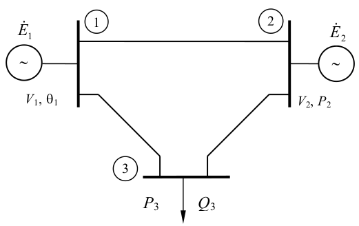
Escrever as equações do fluxo de potência para o sistema da figura.

Equações do flxo de potência:

$\small \begin{array}{*{20}{c}} { P_i = { { | V_i | \sum\limits_{j = 1}^{n} { \left\{ { | V_j | G_{ij} cos \left({ \theta_{ij} }\right) + | V_j | B_{ij} sen \left({ \theta_{ij} }\right) } \right\} }} } ; }&{ i = 1, \cdots, n } \end{array} $

$\small \begin{array}{*{20}{c}} { Q_i = { { | V_i | \sum\limits_{j = 1}^{n} { \left\{ { | V_j | G_{ij} sen \left({ \theta_{ij} }\right) - | V_j | B_{ij} cos \left({ \theta_{ij} }\right) } \right\} }} } ; }&{ i = 1, \cdots, n } \end{array} $

Resolvendo para cada uma das barras do sistema:

$\scriptsize \begin{array}{*{20}{c}} \begin{array}{l} {P_1} = \left| {{V_1}} \right|\left[ {{V_1}\left\{ {{G_{11}}\cos \left( {{\theta _{11}}} \right) + {B_{11}}sen\left( {{\theta _{11}}} \right)} \right\} + } \right.\\ \begin{array}{*{20}{c}} {}&{\left. {{V_2}\left\{ {{G_{12}}\cos \left( {{\theta _{12}}} \right) + {B_{12}}sen\left( {{\theta _{12}}} \right)} \right\} + {V_3}\left\{ {{G_{13}}\cos \left( {{\theta _{13}}} \right) + {B_{13}}sen\left( {{\theta _{13}}} \right)} \right\}} \right]} \end{array} \end{array}\\ \begin{array}{l} {P_2} = \left| {{V_2}} \right|\left[ {{V_1}\left\{ {{G_{21}}\cos \left( {{\theta _{21}}} \right) + {B_{21}}sen\left( {{\theta _{21}}} \right)} \right\} + } \right.\\ \begin{array}{*{20}{c}} {}&{\left. {{V_2}\left\{ {{G_{22}}\cos \left( {{\theta _{22}}} \right) + {B_{22}}sen\left( {{\theta _{22}}} \right)} \right\} + {V_3}\left\{ {{G_{23}}\cos \left( {{\theta _{23}}} \right) + {B_{23}}sen\left( {{\theta _{23}}} \right)} \right\}} \right]} \end{array} \end{array}\\ \begin{array}{l} {P_3} = \left| {{V_3}} \right|\left[ {{V_3}\left\{ {{G_{31}}\cos \left( {{\theta _{31}}} \right) + {B_{31}}sen\left( {{\theta _{31}}} \right)} \right\} + } \right.\\ \begin{array}{*{20}{c}} {}&{\left. {{V_2}\left\{ {{G_{32}}\cos \left( {{\theta _{32}}} \right) + {B_{32}}sen\left( {{\theta _{32}}} \right)} \right\} + {V_3}\left\{ {{G_{33}}\cos \left( {{\theta _{33}}} \right) + {B_{33}}sen\left( {{\theta _{33}}} \right)} \right\}} \right]} \end{array} \end{array} \end{array} $

$\scriptsize \begin{array}{*{20}{c}} \begin{array}{l} {Q_1} = \left| {{V_1}} \right|\left[ {{V_1}\left\{ {{G_{11}}sen\left( {{\theta _{11}}} \right) - {B_{11}}\cos \left( {{\theta _{11}}} \right)} \right\} + } \right.\\ \begin{array}{*{20}{c}} {}&{\left. {{V_2}\left\{ {{G_{12}}\cos \left( {{\theta _{12}}} \right) - {B_{12}}\cos \left( {{\theta _{12}}} \right)} \right\} + {V_3}\left\{ {{G_{13}}sen\left( {{\theta _{13}}} \right) - {B_{13}}\cos \left( {{\theta _{13}}} \right)} \right\}} \right]} \end{array} \end{array}\\ \begin{array}{l} {Q_2} = \left| {{V_2}} \right|\left[ {{V_1}\left\{ {{G_{21}}sen\left( {{\theta _{21}}} \right) - {B_{21}}\cos \left( {{\theta _{21}}} \right)} \right\} + } \right.\\ \begin{array}{*{20}{c}} {}&{\left. {{V_2}\left\{ {{G_{22}}\cos \left( {{\theta _{22}}} \right) - {B_{22}}\cos \left( {{\theta _{22}}} \right)} \right\} + {V_3}\left\{ {{G_{23}}sen\left( {{\theta _{23}}} \right) - {B_{23}}\cos \left( {{\theta _{23}}} \right)} \right\}} \right]} \end{array} \end{array}\\ \begin{array}{l} {Q_3} = \left| {{V_3}} \right|\left[ {{V_3}\left\{ {{G_{31}}sen\left( {{\theta _{31}}} \right) - {B_{31}}\cos \left( {{\theta _{31}}} \right)} \right\} + } \right.\\ \begin{array}{*{20}{c}} {}&{\left. {{V_2}\left\{ {{G_{32}}sen\left( {{\theta _{32}}} \right) - {B_{32}}\cos \left( {{\theta _{32}}} \right)} \right\} + {V_3}\left\{ {{G_{33}}sen\left( {{\theta _{33}}} \right) - {B_{33}}\cos \left( {{\theta _{33}}} \right)} \right\}} \right]} \end{array} \end{array} \end{array}$

Fluxo de Potência - Método Newton-Raphson

Devido à variedade de tipos de barra, o sistema de equações que descreve o sistema elétrico é dividido em dois subsistemas:

Subsistema 1: Este subsistema contém as equações que devem ser resolvidas para se encontrar a solução do fluxo de potência, ou seja, módulo e ângulo das tensões nas barras:

$\small P_i = P_i (|V|, \theta)$; $\small i \in \{ PQ, PV \}$ $\small \rightarrow$ Barras de carga e de tensão controlada.
$\small Q_i = Q_i (|V|, \theta)$; $\small i \in \{ PQ \}$ $\small \rightarrow$ Barras de carga.

Subsistema 2: As incógnitas aqui contidas são determinadas por substituição das variáveis calculadas no Subsistema 1:

$\small P_i = P_i (|V|, \theta)$; $\small i \in \{ V \theta \}$ $\small \rightarrow$ Barra de folga.
$\small Q_i = Q_i (|V|, \theta)$; $\small i \in \{ V \theta, PV \}$ $\small \rightarrow$ Barra de folga e barras de tensão controlada.

Fluxo de Potência - Método Newton-Raphson - Exemplo 3.2.2

Escrever as equações do sistema da figura, separando-as nos subsistemas 1 e 2.

Equações do flxo de potência para o Subsistema 1 ($\small P$ para barras tipo $\small PQ$ e $\small PV$, e $\small Q$ para barras tipo $\small PQ$) :

$\scriptsize \begin{array}{*{20}{c}} \begin{array}{l} {P_2} = \left| {{V_2}} \right|\left[ {{V_1}\left\{ {{G_{21}}\cos \left( {{\theta _{21}}} \right) + {B_{21}}sen\left( {{\theta _{21}}} \right)} \right\} + } \right.\\ \begin{array}{*{20}{c}} {}&{\left. {{V_2}\left\{ {{G_{22}}\cos \left( {{\theta _{22}}} \right) + {B_{22}}sen\left( {{\theta _{22}}} \right)} \right\} + {V_3}\left\{ {{G_{23}}\cos \left( {{\theta _{23}}} \right) + {B_{23}}sen\left( {{\theta _{23}}} \right)} \right\}} \right]} \end{array} \end{array}\\ \begin{array}{l} {P_3} = \left| {{V_3}} \right|\left[ {{V_3}\left\{ {{G_{31}}\cos \left( {{\theta _{31}}} \right) + {B_{31}}sen\left( {{\theta _{31}}} \right)} \right\} + } \right.\\ \begin{array}{*{20}{c}} {}&{\left. {{V_2}\left\{ {{G_{32}}\cos \left( {{\theta _{32}}} \right) + {B_{32}}sen\left( {{\theta _{32}}} \right)} \right\} + {V_3}\left\{ {{G_{33}}\cos \left( {{\theta _{33}}} \right) + {B_{33}}sen\left( {{\theta _{33}}} \right)} \right\}} \right]} \end{array} \end{array} \\ \begin{array}{l} {Q_3} = \left| {{V_3}} \right|\left[ {{V_3}\left\{ {{G_{31}}sen\left( {{\theta _{31}}} \right) - {B_{31}}\cos \left( {{\theta _{31}}} \right)} \right\} + } \right.\\ \begin{array}{*{20}{c}} {}&{\left. {{V_2}\left\{ {{G_{32}}sen\left( {{\theta _{32}}} \right) - {B_{32}}\cos \left( {{\theta _{32}}} \right)} \right\} + {V_3}\left\{ {{G_{33}}sen\left( {{\theta _{33}}} \right) - {B_{33}}\cos \left( {{\theta _{33}}} \right)} \right\}} \right]} \end{array} \end{array} \end{array} $

A solução das três equações acima fornece $\small V_3$, $\small \theta_2$, $\small \theta_3$.

Equações do flxo de potência para o Subsistema 2 ($\small P$ para a barra tipo $\small V \theta$, e $\small Q$ para a barra tipo $\small V \theta$ e as barras tipo $\small PV$):

$\scriptsize \begin{array}{*{20}{c}} \begin{array}{l} {P_1} = \left| {{V_1}} \right|\left[ {{V_1}\left\{ {{G_{11}}\cos \left( {{\theta _{11}}} \right) + {B_{11}}sen\left( {{\theta _{11}}} \right)} \right\} + } \right.\\ \begin{array}{*{20}{c}} {}&{\left. {{V_2}\left\{ {{G_{12}}\cos \left( {{\theta _{12}}} \right) + {B_{12}}sen\left( {{\theta _{12}}} \right)} \right\} + {V_3}\left\{ {{G_{13}}\cos \left( {{\theta _{13}}} \right) + {B_{13}}sen\left( {{\theta _{13}}} \right)} \right\}} \right]} \end{array} \end{array}\\ \begin{array}{l} {Q_1} = \left| {{V_1}} \right|\left[ {{V_1}\left\{ {{G_{11}}sen\left( {{\theta _{11}}} \right) - {B_{11}}\cos \left( {{\theta _{11}}} \right)} \right\} + } \right.\\ \begin{array}{*{20}{c}} {}&{\left. {{V_2}\left\{ {{G_{12}}\cos \left( {{\theta _{12}}} \right) - {B_{12}}\cos \left( {{\theta _{12}}} \right)} \right\} + {V_3}\left\{ {{G_{13}}sen\left( {{\theta _{13}}} \right) - {B_{13}}\cos \left( {{\theta _{13}}} \right)} \right\}} \right]} \end{array} \end{array}\\ \begin{array}{l} {Q_3} = \left| {{V_3}} \right|\left[ {{V_3}\left\{ {{G_{31}}sen\left( {{\theta _{31}}} \right) - {B_{31}}\cos \left( {{\theta _{31}}} \right)} \right\} + } \right.\\ \begin{array}{*{20}{c}} {}&{\left. {{V_2}\left\{ {{G_{32}}sen\left( {{\theta _{32}}} \right) - {B_{32}}\cos \left( {{\theta _{32}}} \right)} \right\} + {V_3}\left\{ {{G_{33}}sen\left( {{\theta _{33}}} \right) - {B_{33}}\cos \left( {{\theta _{33}}} \right)} \right\}} \right]} \end{array} \end{array} \end{array} $

Para determinar as outras variáveis, do Subsistema 2, basta substituir as variáveis calculadas no Subsistema 1 nas equações acima.

Fluxo de Potência - Método Newton-Raphson

Definindo os "resíduos de potência" como:

$\small \begin{array}{*{20}{c}} { \Delta P_i = P_i^{esp} - P_i^{cal} (|V|, \theta); }&{ i \in \{ PQ, PV \} } \end{array} $

$\small \begin{array}{*{20}{c}} { \Delta Q_i = Q_i^{esp} - Q_i^{cal} (|V|, \theta); }&{ i \in \{ PQ \} } \end{array} $

o sistema a ser resolvido pelo Método de Newton-Raphson é:

$\small \begin{array}{*{20}{c}} { \Delta P = 0; }&{ i \in \{ PQ, PV \} } \end{array} $

$\small \begin{array}{*{20}{c}} { \Delta Q = 0; }&{ i \in \{ PQ \} } \end{array} $

Considera-se então o sistema com $\small n$ barras, sendo que:

Barras $\small PQ$: barras de 1 até $\small l$ ($\small n_{PQ} = l$).
Barras $\small PV$: barras de $\small l$ + 1 até $\small n$ - 1 ($\small n_{PV} = n - l - 1$).
Barras $\small V \theta$: barra $\small n$ ($\small n_{V \theta} = 1$).

Fluxo de Potência - Método Newton-Raphson

Relembrando, do Método de Newton-Raphson, na forma geral, tem-se que:

$\small \Delta X^{(k)} = \left[{ J^{(k)} }\right] ^{-1} \Delta C^{(k)} $

A atualização das variáveis usando o Método de Newton-Raphson, para o sistema $\small n$ dimensional, é:

$\small X^{(k + 1)} = X^{(k)} + \Delta X^{(k)} $

Sendo:

$\tiny \Delta {X^{(k)}} = \left[ {\begin{array}{*{20}{c}} {\Delta x_1^{(k)}}\\ {\Delta x_2^{(k)}}\\ \vdots \\ {\Delta x_n^{(k)}} \end{array}} \right];{\rm{ }}\Delta {C^{(k)}} = \left[ {\begin{array}{*{20}{c}} {{c_1} - {{\left( {{f_1}} \right)}^{(k)}}}\\ {{c_2} - {{\left( {{f_2}} \right)}^{(k)}}}\\ \vdots \\ {{c_n} - {{\left( {{f_n}} \right)}^{(k)}}} \end{array}} \right];{\rm{ }}{J^{(k)}} = \left[ {\begin{array}{*{20}{c}} {{{\left( {\frac{{\partial {f_1}}}{{\partial {x_1}}}} \right)}^{(k)}}}&{{{\left( {\frac{{\partial {f_1}}}{{\partial {x_{`2}}}}} \right)}^{(k)}}}& \cdots &{{{\left( {\frac{{\partial {f_1}}}{{\partial {x_n}}}} \right)}^{(k)}}}\\ {{{\left( {\frac{{\partial {f_2}}}{{\partial {x_1}}}} \right)}^{(k)}}}&{{{\left( {\frac{{\partial {f_2}}}{{\partial {x_{`2}}}}} \right)}^{(k)}}}& \cdots &{{{\left( {\frac{{\partial {f_2}}}{{\partial {x_n}}}} \right)}^{(k)}}}\\ \vdots & \vdots & \ddots & \vdots \\ {{{\left( {\frac{{\partial {f_n}}}{{\partial {x_1}}}} \right)}^{(k)}}}&{{{\left( {\frac{{\partial {f_n}}}{{\partial {x_{`2}}}}} \right)}^{(k)}}}& \cdots &{{{\left( {\frac{{\partial {f_n}}}{{\partial {x_n}}}} \right)}^{(k)}}} \end{array}} \right]$

Fluxo de Potência - Método Newton-Raphson

Nas expressões:

$\small \Delta X^{(k)} = \left[{ J^{(k)} }\right] ^{-1} \Delta C^{(k)} $

$\small X^{(k + 1)} = X^{(k)} + \Delta X^{(k)} $

Podem-se usar, para o Subsistema 1, as seguintes relações:

$\scriptsize \Delta C^{(k)} = {\left[ {\begin{array}{*{20}{c}} {\Delta {P_1}}&{\Delta {P_2}}& \cdots &{\Delta {P_l}}&{\Delta {P_{l + 1}}}& \cdots &{\Delta {P_{n - 1}}}&{\Delta {Q_1}}&{\Delta {Q_2}}& \cdots &{\Delta {Q_l}} \end{array}} \right]^T} $

$\scriptsize X^{(k)} = {\left[ {\begin{array}{*{20}{c}} {{\theta _1}}&{{\theta _2}}& \cdots &{{\theta _l}}&{{\theta _{l + 1}}}& \cdots &{{\theta _{n - 1}}}&{{V_1}}&{{V_2}}& \cdots &{{V_l}} \end{array}} \right]^T} $

$\scriptsize \Delta X^{(k)} = {\left[ {\begin{array}{*{20}{c}} {{\Delta \theta _1}}&{{\Delta \theta _2}}& \cdots &{{\Delta \theta _l}}&{{\Delta \theta _{l + 1}}}& \cdots &{{\Delta \theta _{n - 1}}}&{{\Delta V_1}}&{{\Delta V_2}}& \cdots &{{\Delta V_l}} \end{array}} \right]^T} $

Fluxo de Potência - Método Newton-Raphson

Ou:

$\scriptsize \Delta C^{(k)} = {\left[ {\begin{array}{*{20}{c}} {\underline {\Delta P} }\\ {\underline {\Delta Q} } \end{array}} \right]^{(k)}} $

$\scriptsize X^{(k)} = {\left[ {\begin{array}{*{20}{c}} {\underline \theta }\\ {\underline V } \end{array}} \right]^{(k)}} $

$\scriptsize \Delta X^{(k)} = {\left[ {\begin{array}{*{20}{c}} {\underline {\Delta \theta} }\\ {\underline {\Delta V} } \end{array}} \right]^{(k)}} $

Fluxo de Potência - Método Newton-Raphson

$\scriptsize \Delta C^{(k)} = {\left[ {\begin{array}{*{20}{c}} {\underline {\Delta P} }\\ {\underline {\Delta Q} } \end{array}} \right]^{(k)}} $

$\scriptsize X^{(k)} = {\left[ {\begin{array}{*{20}{c}} {\underline \theta }\\ {\underline V } \end{array}} \right]^{(k)}} $

$\scriptsize \Delta X^{(k)} = {\left[ {\begin{array}{*{20}{c}} {\underline {\Delta \theta} }\\ {\underline {\Delta V} } \end{array}} \right]^{(k)}} $

Assim, tem-se que:

$\small \Delta X^{(k)} = \left[{ J^{(k)} }\right] ^{-1} \Delta C^{(k)} $

$\small {\left[ {\begin{array}{*{20}{c}} {\underline {\Delta \theta } }\\ {\underline {\Delta V} } \end{array}} \right]^{(k)}} = \left[{ J^{(k)} }\right] ^{-1} {\left[ {\begin{array}{*{20}{c}} {\underline {\Delta P} }\\ {\underline {\Delta Q} } \end{array}} \right]^{(k)}} $

Fluxo de Potência - Método Newton-Raphson

A atualização das variáveis, na solução do Subsistema 1, é então:

$\small {\left[ {\begin{array}{*{20}{c}} {\underline \theta }\\ {\underline V } \end{array}} \right]^{(k + 1)}} = {\left[ {\begin{array}{*{20}{c}} {\underline \theta }\\ {\underline V } \end{array}} \right]^{(k)}} + {\left[ {\begin{array}{*{20}{c}} {\underline {\Delta \theta } }\\ {\underline {\Delta V} } \end{array}} \right]^{(k)}} $

A convergência é conferida de acordo com:

$\small \left\{ {\left| {\underline {\Delta P} } \right|} \right\} \le {\varepsilon _P} $

$\small \left\{ {\left| {\underline {\Delta Q} } \right|} \right\} \le {\varepsilon _Q} $

Fluxo de Potência - Método Newton-Raphson

$\small {\left[ {\begin{array}{*{20}{c}} {\underline {\Delta P} }\\ {\underline {\Delta Q} } \end{array}} \right]^{(k)}} = \left[{ J^{(k)} }\right] {\left[ {\begin{array}{*{20}{c}} {\underline {\Delta \theta } }\\ {\underline {\Delta V} } \end{array}} \right]^{(k)}} $

Decompondo a matriz Jacobiana (lembrando que $\small n_{PQ} = l$ e $\small n_{PV} = n - l - 1$):

$\small {J_{(n + l - 1)(n + l - 1)}} = \left[ {\begin{array}{*{20}{c}} {{{\partial \underline {\Delta P} }}/{{\partial \underline \theta }}}&{{{\partial \underline {\Delta P} }}/{{\partial \underline V }}}\\ {{{\partial \underline {\Delta Q} }}/{{\partial \underline \theta }}}&{{{\partial \underline {\Delta Q} }}/{{\partial \underline V }}} \end{array}} \right] $

Fluxo de Potência - Método Newton-Raphson

$\scriptsize {J_{(n + l - 1)(n + l - 1)}} = \left[ {\begin{array}{*{20}{c}} {{{\partial \underline {\Delta P} }}/{{\partial \underline \theta }}}&{{{\partial \underline {\Delta P} }}/{{\partial \underline V }}}\\ {{{\partial \underline {\Delta Q} }}/{{\partial \underline \theta }}}&{{{\partial \underline {\Delta Q} }}/{{\partial \underline V }}} \end{array}} \right] $

Lembrando que:

$\scriptsize \Delta P_i = P_i^{esp} - P_i^{cal} (|V|, \theta) = P_i^{esp} - P_i^{cal} $

$\scriptsize \Delta Q_i = Q_i^{esp} - Q_i^{cal} (|V|, \theta) = Q_i^{esp} - Q_i^{cal} $

então:

$\small \begin{array}{*{20}{c}} { \frac{{\partial {\Delta P_i} }}{{\partial \ \theta_j }} = \frac{{\partial \left( {\underline {{P_i^{esp}}} - \underline {{P_i^{cal}}} } \right)}}{{\partial \theta_j }} = \frac{{\partial { {P_i^{cal}}} }}{{\partial \theta_j }} = \frac{{\partial { P_i} }}{{\partial \theta_j }} ;}&{ \frac{{\partial {\Delta P_i} }}{{\partial \ V_j }} = \frac{{\partial \left( {\underline {{P_i^{esp}}} - \underline {{P_i^{cal}}} } \right)}}{{\partial V_j }} = \frac{{\partial { {P_i^{cal}}} }}{{\partial V_j }} = \frac{{\partial { P_i} }}{{\partial V_j }} }\\ { \frac{{\partial {\Delta Q_i} }}{{\partial \ \theta_j }} = \frac{{\partial \left( {\underline {{Q_i^{esp}}} - \underline {{Q_i^{cal}}} } \right)}}{{\partial \theta_j }} = \frac{{\partial { {Q_i^{cal}}} }}{{\partial \theta_j }} = \frac{{\partial { Q_i} }}{{\partial \theta_j }} ;}&{ \frac{{\partial {\Delta Q_i} }}{{\partial \ V_j }} = \frac{{\partial \left( {\underline {{Q_i^{esp}}} - \underline {{Q_i^{cal}}} } \right)}}{{\partial V_j }} = \frac{{\partial { {Q_i^{cal}}} }}{{\partial V_j }} = \frac{{\partial { Q_i} }}{{\partial V_j }} } \end{array} $

Fluxo de Potência - Método Newton-Raphson

Assim, tem-se que:

ou:

$\small {J_{(n + l - 1)(n + l - 1)}} = \left[ {\begin{array}{*{20}{c}} {{{\partial \underline { P} }}/{{\partial \underline \theta }}}&{{{\partial \underline { P} }}/{{\partial \underline V }}}\\ {{{\partial \underline { Q} }}/{{\partial \underline \theta }}}&{{{\partial \underline { Q} }}/{{\partial \underline V }}} \end{array}} \right] $

Fluxo de Potência - Método Newton-Raphson

Expandindo a matriz Jacobiana, tem-se que:

$\scriptsize \begin{array}{l} {J_{(n - 1 + l)(n - 1 + l)}} = \left[ {\begin{array}{*{20}{c}} {\frac{{\partial {P_1}}}{{\partial {\theta _1}}}}&{\frac{{\partial {P_1}}}{{\partial {\theta _2}}}}& \cdots &{\frac{{\partial {P_1}}}{{\partial {\theta _{n - 1}}}}}&|&{\frac{{\partial {P_1}}}{{\partial {V_1}}}}&{\frac{{\partial {P_1}}}{{\partial {V_2}}}}& \cdots &{\frac{{\partial {P_1}}}{{\partial {V_l}}}}\\ {\frac{{\partial {P_2}}}{{\partial {\theta _1}}}}&{\frac{{\partial {P_2}}}{{\partial {\theta _2}}}}& \cdots &{\frac{{\partial {P_2}}}{{\partial {\theta _{n - 1}}}}}&|&{\frac{{\partial {P_2}}}{{\partial {V_1}}}}&{\frac{{\partial {P_2}}}{{\partial {V_2}}}}& \cdots &{\frac{{\partial {P_2}}}{{\partial {V_l}}}}\\ \vdots & \vdots &H& \vdots &|& \vdots & \vdots &N& \vdots \\ {\frac{{\partial {P_{n - 1}}}}{{\partial {\theta _1}}}}&{\frac{{\partial {P_{n - 1}}}}{{\partial {\theta _2}}}}& \cdots &{\frac{{\partial {P_{n - 1}}}}{{\partial {\theta _{n - 1}}}}}&|&{\frac{{\partial {P_{n - 1}}}}{{\partial {V_1}}}}&{\frac{{\partial {P_{n - 1}}}}{{\partial {V_2}}}}& \cdots &{\frac{{\partial {P_{n - 1}}}}{{\partial {V_l}}}}\\ {--}&{--}&{--}&{--}&|&{--}&{--}&{--}&{--}\\ {\frac{{\partial {Q_1}}}{{\partial {\theta _1}}}}&{\frac{{\partial {Q_1}}}{{\partial {\theta _2}}}}& \cdots &{\frac{{\partial {Q_1}}}{{\partial {\theta _{n - 1}}}}}&|&{\frac{{\partial {Q_1}}}{{\partial {V_1}}}}&{\frac{{\partial {Q_1}}}{{\partial {V_2}}}}& \cdots &{\frac{{\partial {Q_1}}}{{\partial {V_l}}}}\\ {\frac{{\partial {Q_2}}}{{\partial {\theta _1}}}}&{\frac{{\partial {Q_2}}}{{\partial {\theta _2}}}}& \cdots &{\frac{{\partial {Q_2}}}{{\partial {\theta _{n - 1}}}}}&|&{\frac{{\partial {Q_2}}}{{\partial {V_1}}}}&{\frac{{\partial {Q_2}}}{{\partial {V_2}}}}& \cdots &{\frac{{\partial {Q_2}}}{{\partial {V_l}}}}\\ \vdots & \vdots &M& \vdots &|& \vdots & \vdots &L& \vdots \\ {\frac{{\partial {Q_l}}}{{\partial {\theta _1}}}}&{\frac{{\partial {Q_l}}}{{\partial {\theta _2}}}}& \cdots &{\frac{{\partial {Q_l}}}{{\partial {\theta _{n - 1}}}}}&|&{\frac{{\partial {Q_l}}}{{\partial {V_1}}}}&{\frac{{\partial {Q_l}}}{{\partial {V_2}}}}& \cdots &{\frac{{\partial {Q_l}}}{{\partial {V_l}}}} \end{array}} \right] \end{array} $

Fluxo de Potência - Método Newton-Raphson

$\small {J_{(n + l - 1)(n + l - 1)}} = \left[ {\begin{array}{*{20}{c}} {H}&{N}\\ {M}&{L} \end{array}} \right] $

$\small {H_{(n - 1)(n - 1)}} = \partial \underline P /\partial \underline \theta $

$\small {N_{(n - 1)(l)}} = \partial \underline P /\partial \underline V $

$\small {M_{(n - 1)(n - 1)}} = \partial \underline Q /\partial \underline \theta $

$\small {L_{(n - 1)(l)}} = \partial \underline Q /\partial \underline V $

Fluxo de Potência - Método Newton-Raphson

Elementos da matriz $\small H$:

$\small \left\{ \begin{array}{l} {H_{ii}} = \frac{\partial P_i}{\partial \theta_i} = - {B_{ii}}V_i^2 - {V_i}\sum\limits_{j \in {\Omega _i}} {{V_j}\left( {{G_{ij}} sen{\theta _{ij}} - {B_{ij}} cos {\theta _{ij}}} \right)} \\ \begin{array}{*{20}{c}} {}& = \end{array} - {B_{ii}}V_i^2 - {Q_i}\\ {H_{ij}} = \frac{\partial P_i}{\partial \theta_j} = {V_i}{V_j}\left( {{G_{ij}} sen{\theta _{ij}} - {B_{ij}} cos {\theta _{ij}}} \right)\\ {H_{ji}} = \frac{\partial P_j}{\partial \theta_i} = - {V_i}{V_j}\left( {{G_{ij}} sen{\theta _{ij}} + {B_{ij}} cos {\theta _{ij}}} \right) \end{array} \right. $

$\small \Omega _i$: Barras conectadas à barra $\small i$, excluindo a própria barra $\small i$.

Fluxo de Potência - Método Newton-Raphson

Elementos da matriz $\small N$:

$\small \left\{ \begin{array}{l} {N_{ii}} = \frac{\partial P_i}{\partial V_i} = {G_{ii}}V_i + \sum\limits_{j \in {\Omega _i}} {{V_j}\left( {{G_{ij}} cos{\theta _{ij}} + {B_{ij}} sen {\theta _{ij}}} \right)} \\ \begin{array}{*{20}{c}} {}& = \end{array} V_i^{-1} \left({ P_i + G_{ii}V_i^2 }\right)\\ {N_{ij}} = \frac{\partial P_i}{\partial V_j} = {V_i}\left( {{G_{ij}} cos{\theta _{ij}} + {B_{ij}} sen {\theta _{ij}}} \right)\\ {N_{ji}} = \frac{\partial P_j}{\partial V_i} = {V_j}\left( {{G_{ij}} cos{\theta _{ij}} - {B_{ij}} sen {\theta _{ij}}} \right) \end{array} \right. $

$\small \Omega _i$: Barras conectadas à barra $\small i$, excluindo a própria barra $\small i$.

Fluxo de Potência - Método Newton-Raphson

Elementos da matriz $\small M$:

$\small \left\{ \begin{array}{l} {M_{ii}} = \frac{\partial Q_i}{\partial \theta_i} = - {G_{ii}}V_i^2 + {V_i}\sum\limits_{j \in {\Omega _i}} {{V_j}\left( {{G_{ij}} cos{\theta _{ij}} + {B_{ij}} sen {\theta _{ij}}} \right)} \\ \begin{array}{*{20}{c}} {}& = \end{array} - {G_{ii}}V_i^2 + {P_i}\\ {M_{ij}} = \frac{\partial Q_i}{\partial \theta_j} = - {V_i}{V_j}\left( {{G_{ij}} cos{\theta _{ij}} + {B_{ij}} sen {\theta _{ij}}} \right)\\ {M_{ji}} = \frac{\partial Q_j}{\partial \theta_i} = - {V_i}{V_j}\left( {{G_{ij}} cos{\theta _{ij}} - {B_{ij}} sen {\theta _{ij}}} \right) \end{array} \right. $

$\small \Omega _i$: Barras conectadas à barra $\small i$, excluindo a própria barra $\small i$.

Fluxo de Potência - Método Newton-Raphson

Elementos da matriz $\small L$:

$\small \left\{ \begin{array}{l} {L_{ii}} = \frac{\partial Q_i}{\partial V_i} = - {B_{ii}}V_i + \sum\limits_{j \in {\Omega _i}} {{V_j}\left( {{G_{ij}} sen{\theta _{ij}} - {B_{ij}} cos {\theta _{ij}}} \right)} \\ \begin{array}{*{20}{c}} {}& = \end{array} V_i^{-1} \left({ Q_i - B_{ii}V_i^2 }\right)\\ {L_{ij}} = \frac{\partial Q_i}{\partial V_j} = {V_i}\left( {{G_{ij}} sen{\theta _{ij}} - {B_{ij}} cos {\theta _{ij}}} \right)\\ {L_{ji}} = \frac{\partial Q_j}{\partial V_i} = - {V_j}\left( {{G_{ij}} sen{\theta _{ij}} + {B_{ij}} cos {\theta _{ij}}} \right) \end{array} \right. $

$\small \Omega _i$: Barras conectadas à barra $\small i$, excluindo a própria barra $\small i$.

Fluxo de Potência - Método Newton-Raphson

Resumo do equacionamento:

$\scriptsize P_i = { { | V_i | \sum\limits_{j = 1}^{n} { \left\{ { | V_j | G_{ij} cos \left({ \theta_{ij} }\right) + | V_j | B_{ij} sen \left({ \theta_{ij} }\right) } \right\} }} } $

$\scriptsize Q_i = { { | V_i | \sum\limits_{j = 1}^{n} { \left\{ { | V_j | G_{ij} sen \left({ \theta_{ij} }\right) - | V_j | B_{ij} cos \left({ \theta_{ij} }\right) } \right\} }} } $

$\tiny {\left[ {\begin{array}{*{20}{c}} {\underline {\Delta P} }\\ {\underline {\Delta Q} } \end{array}} \right]^{(k)}} = \left[ {\begin{array}{*{20}{c}} {H}&{N}\\ {M}&{L} \end{array}} \right] ^{(k)} {\left[ {\begin{array}{*{20}{c}} {\underline {\Delta \theta } }\\ {\underline {\Delta V} } \end{array}} \right]^{(k)}} $

$\tiny {\left[ {\begin{array}{*{20}{c}} {\underline { \theta } }\\ {\underline { V} } \end{array}} \right]^{(k + 1)}} = {\left[ {\begin{array}{*{20}{c}} {\underline { \theta } }\\ {\underline { V} } \end{array}} \right]^{(k)}} + {\left[ {\begin{array}{*{20}{c}} {\underline {\Delta \theta } }\\ {\underline {\Delta V} } \end{array}} \right]^{(k)}} $

Fluxo de Potência - Método Newton-Raphson

Algoritmo do Método Newton-Raphson:

Passo 1: Construir a matriz $\small Y_{\rm{Barra}}$.

Passo 2: Arbitrar valores iniciais das variáveis de estado $\small \underline { \theta}$ para as barras tipo $\small PQ$ e $\small PV$, e $\small \underline { V}$ para as barras tipo $\small PQ$.

Passo 3: Calcular $\small \Delta P_i$ e $\small \Delta Q_i$, de acordo com as seguintes expressões:

$\small \begin{array}{*{20}{c}} { \Delta P_i = P_i^{esp} - P_i^{cal}; }&{ i \in \{ PQ, PV \} } \end{array} $

$\small \begin{array}{*{20}{c}} { \Delta Q_i = Q_i^{esp} - Q_i^{cal}; }&{ i \in \{ PQ \} } \end{array} $

Fluxo de Potência - Método Newton-Raphson

Algoritmo do Método Newton-Raphson:

$\small \begin{array}{*{20}{c}} { \Delta P_i = P_i^{esp} - P_i^{cal} (|V|, \theta); }&{ i \in \{ PQ, PV \} } \end{array} $

$\small \begin{array}{*{20}{c}} { \Delta Q_i = Q_i^{esp} - Q_i^{cal} (|V|, \theta); }&{ i \in \{ PQ \} } \end{array} $

Se:

$\small \left\{ {\left| {\underline {\Delta P} } \right|} \right\} \le {\varepsilon _P} $
$\small \left\{ {\left| {\underline {\Delta Q} } \right|} \right\} \le {\varepsilon _Q} $

então parar; caso contrário, ir ao Passo 4.

Fluxo de Potência - Método Newton-Raphson

Algoritmo do Método Newton-Raphson:

Passo 4: Fazer $\small k = k + 1$. Montar a matriz Jacobiana $\small J^{(k)}$.

Passo 5: Solucionar o sistema linearizado:

$\small {\left[ {\begin{array}{*{20}{c}} {\underline {\Delta P} }\\ {\underline {\Delta Q} } \end{array}} \right]^{(k)}} = J ^{(k)} {\left[ {\begin{array}{*{20}{c}} {\underline {\Delta \theta } }\\ {\underline {\Delta V} } \end{array}} \right]^{(k)}} $

Passo 6: Atualizar a solução do problema:

$\small {\left[ {\begin{array}{*{20}{c}} {\underline { \theta } }\\ {\underline { V} } \end{array}} \right]^{(k + 1)}} = {\left[ {\begin{array}{*{20}{c}} {\underline { \theta } }\\ {\underline { V} } \end{array}} \right]^{(k)}} + {\left[ {\begin{array}{*{20}{c}} {\underline {\Delta \theta } }\\ {\underline {\Delta V} } \end{array}} \right]^{(k)}} $

Passo 7: Voltar ao Passo 3.

Fluxo de Potência - Método Newton-Raphson - Exemplo 3.3.3

Usar o Método Newton-Raphson, considerando como solução inicial $\small \theta_2^{(0)} = 0$ e tolerância em $\small \Delta P = \epsilon = 0,003$, para para resolver o problema de fluxo de potência do sistema elétrico da figura a seguir (dados em pu):

Dados das barras:

Dados da linha:

Montagem da matriz $\small Y_{\rm{Barra}}$:

$\small Y_{12} = \frac{1}{0,0 + j1,0} = 0,19 - j0,96$

$\small Y_{\rm{Barra}} = \left[ {\begin{array}{*{20}{c}} {0,19 - j0,94}&{ - 0,19 + j0,96}\\ { - 0,19 + j0,96}&{0,19 - j0,94} \end{array}} \right]$

Dados das barras:

$\small Y_{\rm{Barra}} = \left[ {\begin{array}{*{20}{c}} {0,19 - j0,94}&{ - 0,19 + j0,96}\\ { - 0,19 + j0,96}&{0,19 - j0,94} \end{array}} \right]$

$\small Y_{\rm{Barra}} = G_{\rm{Barra}} + jB_{\rm{Barra}}$

$\small G_{\rm{Barra}} = \left[ {\begin{array}{*{20}{c}} {0,19 }&{ - 0,19 }\\ { - 0,19 }&{0,19 } \end{array}} \right]$

$\small B_{\rm{Barra}} = \left[ {\begin{array}{*{20}{c}} { - j0,94}&{ j0,96}\\ { j0,96}&{9 - j0,94} \end{array}} \right]$

Solução do Subsistema 1 (não há barras tipo $\small PQ$; portanto, limita-se à solução de $\small \theta$ para a barra tipo $PV$):

Teste de convergência:

$\small P_i = { { | V_i | \sum\limits_{j = 1}^{n} { \left\{ { | V_j | G_{ij} cos \left({ \theta_{ij} }\right) + | V_j | B_{ij} sen \left({ \theta_{ij} }\right) } \right\} }} }$

$\small P_2 = | V_2 | \left\{ { | V_1 | G_{21} cos \left({ \theta_{21} }\right) + | V_1 | B_{21} sen \left({ \theta_{21} }\right) } \right\} + $
$\small | V_2 | \left\{ { | V_2 | G_{22} cos \left({ \theta_{22} }\right) + | V_2 | B_{22} sen \left({ \theta_{22} }\right) } \right\} $

$\small P_2^{(0)} = 0,00$

$\small \Delta P_2^{(0)} = P_2^{esp} - P_2^{cal,(0)} = -0,4 - P_2^{(0)} = - 0,40$

$\small | \Delta P_2^{(0)} | > \epsilon$ $\leftarrow$ Não convergiu.

Processo iterativo pelo Método Newton-Raphson:

Primeira iteração $\small k = 1$:

$\small \Delta P_2^{(1)} = -J^{(1)} \Delta \theta_2^{(1)} $

$\small \Delta P_2^{(1)} = H^{(1)} \Delta \theta_2^{(1)} $

$\small H_{22}^{(1)} = -| V_2 |^2 B_{22} - | V_2 | \left\{ { | V_1 | G_{21} sen \left({ \theta_{21} }\right) - | V_1 | B_{21} cos \left({ \theta_{21} }\right) } \right\} + $
$\small | V_2 | \left\{ { | V_2 | G_{22} sen \left({ \theta_{22} }\right) - | V_2 | B_{22} cos \left({ \theta_{22} }\right) } \right\} $

$\small H_{22}^{(1)} = 0,96$

$\small \Delta P_2^{(1)} = -J^{(1)} \Delta \theta_2^{(1)} $

$\small \Delta P_2^{(1)} = H^{(1)} \Delta \theta_2^{(1)} = H_{22}^{(1)} \Delta \theta_2^{(1)} $

$\small \Delta \theta_{2}^{(1)} = \{ H_{22}^{(1)} \} ^{-1} \Delta P_2^{(1)} = -0,416 $ rad

$\small \theta_{2}^{(1)} = \theta_{2}^{(0)} + \Delta \theta_{2}^{(1)} = 0,00 -0,416 $ rad

$\small P_2^{(1)} = -0,37$ pu

$\small \Delta P_2^{(1)} = P_2^{esp} - P_2^{cal,(1)} = -0,4 - P_2^{(1)} = - 0,03$

$\small | \Delta P_2^{(1)} | > \epsilon$ $\leftarrow$ Não convergiu.

Segunda iteração $\small k = k + 1 = 2$:

$\small \Delta P_2^{(2)} = -J^{(2)} \Delta \theta_2^{(2)} $

$\small \Delta P_2^{(2)} = H^{(2)} \Delta \theta_2^{(2)} $

$\small H_{22}^{(2)} = -| V_2 |^2 B_{22} - | V_2 | \left\{ { | V_1 | G_{21} sen \left({ \theta_{21} }\right) - | V_1 | B_{21} cos \left({ \theta_{21} }\right) } \right\} + $
$\small | V_2 | \left\{ { | V_2 | G_{22} sen \left({ \theta_{22} }\right) - | V_2 | B_{22} cos \left({ \theta_{22} }\right) } \right\} $

$\small H_{22}^{(2)} = 0,80$

$\small \Delta P_2^{(2)} = -J^{(2)} \Delta \theta_2^{(2)} $

$\small \Delta P_2^{(2)} = H^{(2)} \Delta \theta_2^{(2)} = H_{22}^{(2)} \Delta \theta_2^{(2)} $

$\small \Delta \theta_{2}^{(2)} = \{ H_{22}^{(2)} \} ^{-1} \Delta P_2^{(2)} = -0,034 $ rad

$\small \theta_{2}^{(1)} = \theta_{2}^{(0)} + \Delta \theta_{2}^{(1)} = -0,416 - 0,034 = -0,45 $ rad

$\small \theta_{2}^{(1)} = -0,45 $ rad

$\small P_2^{(2)} = -0,399$ pu

$\small \Delta P_2^{(1)} = P_2^{esp} - P_2^{cal,(1)} = -0,4 - P_2^{(1)} = - 0,001$

$\small | \Delta P_2^{(1)} | < \epsilon $ $\leftarrow$ Convergiu!

Solução encontrada para todas as variáveis de estado, ou seja:

$\small V_2 = | V_2^{(2)} | \angle \theta_2^{(2)} = 1,0 \angle -0,45$ rad $\small = 1,0 \angle -25,79^{\circ}$

Solução do Subsistema 2 ($\small P$ e $\small Q$ para a barra tipo $\small V \theta$, e $\small Q$ para a barra tipo $PV$):

$\small P_i = { { | V_i | \sum\limits_{j = 1}^{n} { \left\{ { | V_j | G_{ij} cos \left({ \theta_{ij} }\right) + | V_j | B_{ij} sen \left({ \theta_{ij} }\right) } \right\} }} }$

$\small P_1 = 0,44$ pu

$\small Q_i = { { | V_i | \sum\limits_{j = 1}^{n} { \left\{ { | V_j | G_{ij} sen \left({ \theta_{ij} }\right) - | V_j | B_{ij} cos \left({ \theta_{ij} }\right) } \right\} }} }$

$\small Q_1 = -7,89 \times 10^{-3}$ pu

$\small Q_2 = 0,16$ pu

Fluxo de Potência - Método Newton-Raphson Desacoplado

Este método é baseado no forte acoplamento entre as variáveis $\small Pθ$ e $\small QV$, ou seja $\small \partial \underline P / \partial \underline \theta > > \partial \underline P / \partial \underline V$ e $\small \partial \underline Q / \partial \underline V > > \partial \underline Q / \partial \underline \theta$.

Assim, as matrizes $\small M = \partial \underline P / \partial \underline V$ e $\small N = \partial \underline Q / \partial \underline \theta$ sao desprezadas. O sistema fica então:

$\small {\left[ {\begin{array}{*{20}{c}} {\underline {\Delta P} }\\ {\underline {\Delta Q} } \end{array}} \right]^{(k)}} = \left[ {\begin{array}{*{20}{c}} {H}&{0}\\ {0}&{L} \end{array}} \right] ^{(k)} {\left[ {\begin{array}{*{20}{c}} {\underline {\Delta \theta } }\\ {\underline {\Delta V} } \end{array}} \right]^{(k)}} $

Dessa forma, sao definidos dois sistemas de equaçoes:

$\small {\left[ {\begin{array}{*{20}{c}} {\underline {\Delta P} } \end{array}} \right]^{(k)}} = \left[ {\begin{array}{*{20}{c}} {H} \end{array}} \right] ^{(k)} {\left[ {\begin{array}{*{20}{c}} {\underline {\Delta \theta } } \end{array}} \right]^{(k)}} $

$\small {\left[ {\begin{array}{*{20}{c}} {\underline {\Delta Q} } \end{array}} \right]^{(k)}} = \left[ {\begin{array}{*{20}{c}} {L} \end{array}} \right] ^{(k)} {\left[ {\begin{array}{*{20}{c}} {\underline {\Delta V } } \end{array}} \right]^{(k)}} $

Fluxo de Potência - Método Newton-Raphson Desacoplado Rápido

Consideraçoes sobre as matrizes $\small H$ e $\small L$. Estas consideraçoes objetivam transformar as matrizes $\small H$ e $\small L$ em matrizes constantes:

Divisão das equações de resíduo pelo respectivo módulo da tensão com a finalidade de acelerar a convergência:

$\small \frac{\Delta P_i}{V_i} = \frac{P_i^{esp} - P_i^{cal} (|V|, \theta)}{V_k}$; $\small k = 1, ..., n-1$

$\small \frac{\Delta Q_i}{V_i} = \frac{Q_i^{esp} - Q_i^{cal} (|V|, \theta)}{V_k}$; $\small k = 1, ..., l$

O sistema fica então:

$\small \left\{ \begin{array}{l} {\left[ {\underline {\Delta P} /\underline V } \right]^{(k)}} = {\left[ {H'} \right]^{(k)}}{\left[ {\underline {\Delta \theta } } \right]^{(k)}}\\ {\left[ {\underline {\Delta Q} /\underline V } \right]^{(k)}} = {\left[ {L'} \right]^{(k)}}{\left[ {\underline {\Delta V} } \right]^{(k)}} \end{array} \right.$

Fluxo de Potência - Método Newton-Raphson Desacoplado Rápido

As matrizes $\small H'$ e $\small L'$ sao definidas por:

$\small \begin{array}{l} H{'_{ij}} = \frac{{{H_{ij}}}}{{{V_i}}} = {V_j}\left\{ {{G_{ij}}sen\left( {{\theta _{ij}}} \right) - {B_{ij}}cos\left( {{\theta _{ij}}} \right)} \right\}\\ H{'_{ii}} = \frac{{{H_{ii}}}}{{{V_i}}} = - {V_i}{B_{ii}} - \left[ {\sum\limits_{j \in {\Omega _i}} {{V_j}\left\{ {{G_{ij}}sen\left( {{\theta _{ij}}} \right) - {B_{ij}}cos\left( {{\theta _{ij}}} \right)} \right\}} } \right]\\ L{'_{ij}} = \frac{{{L_{ij}}}}{{{V_i}}} = {G_{ij}}sen\left( {{\theta _{ij}}} \right) - {B_{ij}}cos\left( {{\theta _{ij}}} \right)\\ L{'_{ii}} = \frac{{{L_{ii}}}}{{{V_i}}} = - {B_{ii}} + \frac{1}{{{V_k}}}\sum\limits_{j \in {\Omega _i}} {{V_j}\left\{ {{G_{ij}}sen\left( {{\theta _{ij}}} \right) - {B_{ij}}cos\left( {{\theta _{ij}}} \right)} \right\}} \end{array} $

Fluxo de Potência - Método Newton-Raphson Desacoplado Rápido

Hipóteses para o cálculo dos elementos de $\small H'$ e $\small L'$:

Sistema pouco carregado. Com esta consideração, assume-se que $\small \theta_{ij}$ é pequeno e, consequentemente, $\small cos\left( {{\theta _{ij}}} \right) \simeq 1$.
Em linhas de EAT e UAT, a relaçao $\small B_{ij}/G_{ij}$ é alta, de 5 a 20, logo $\small \small B_{ij} >> G_{ij} cos\left( {{\theta _{ij}}} \right)$, ou seja, despreza-se o termo $\small G_{ij} cos\left( {{\theta _{ij}}} \right)$.
As reatâncias transversais nas barras (reatores, capacitores, cargas) são muito maiores do que a reatância série, logo $\small B_{ii} V_i^{2} >> Q_i $.
As tensões $\small V_i$ e $\small V_j$ estão sempre próximas de 1,0 pu.

Fluxo de Potência - Método Newton-Raphson Desacoplado Rápido

Aplicando as considerações anteriores no cálculo dos elementos das matrizes $\small H'$ e $\small L'$, chega-se a:

$\small \begin{array}{l} \left[ {H{'_{ij}}} \right] \cong \left[ { - {B_{ij}}} \right]\\ \left[ {H{'_{ii}}} \right] \cong \left[ { - {B_{ii}}} \right]\\ \left[ {L{'_{ij}}} \right] \cong \left[ { - {B_{ij}}} \right]\\ \left[ {L{'_{ii}}} \right] \cong \left[ { - {B_{ii}}} \right] \end{array} $

Fluxo de Potência - Método Newton-Raphson Desacoplado Rápido

As matrizes de coeficientes se tornam, desta forma, constantes durante todo o processo iterativo, passando a ser chamadas de:

$\small \begin{array}{l} H' \to B'\\ L' \to B'' \end{array} $

Melhorias no desempenho do método são obtidas desprezando as resistências série e as reatâncias shunt na montagem de $\small B'$.

Fluxo de Potência - Método Newton-Raphson Desacoplado Rápido

As considerações anteriores no cálculo dos elementos das matrizes $\small B'$ e $\small B''$ permitem observar que:

Têm estruturas idênticas às das matrizes $\small H$ e $\small L$ e são numericamente simétricas.
São semelhantes à matriz $\small B$ com as seguintes diferenças:
- As linhas e colunas referentes à barra de referência não aparecem em $\small B'$.
- As linhas e colunas referentes à barra de referência e às barras tipo $\small PV$ não aparecem em $\small B''$.
Dependem somente dos parâmetros da rede $\small \rightarrow$ São constantes ao longo do processo iterativo.

Fluxo de Potência - Método Newton-Raphson Desacoplado Rápido

Formulação final do método Desacoplado Rápido:

Os elementos de $\small B'$ e $\small B''$ são definidos como:

$\scriptsize \begin{array}{l} B{'_{ij}} = - \frac{1}{{{x_{ij}}}}\\ B{'_{ii}} = \sum\limits_{j \in {\Omega _i}} {\frac{1}{{{x_{ij}}}}} \\ B'{'_{ij}} = - {B_{ij}}\\ B'{'_{ii}} = - {B_{ii}} \end{array} $
O Metodo de Newton-Raphson Desacoplado Rápido então é formulado como:

$\scriptsize \left\{ \begin{array}{l} {\left[ { \underline{\Delta P} / \underline{V} } \right]} = {\left[ {B'} \right]}{\left[ { \underline{\Delta \theta } } \right]}\\ {\left[ { \underline{\Delta Q} / \underline{V} } \right]} = {\left[ {B''} \right]}{\left[ \underline{\Delta V } \right]} \end{array} \right.$

Fluxo de Potência - Método Newton-Raphson Desacoplado Rápido - Exemplo 3.3.4

Usar o Método Newton-Raphson Desacoplado Rápido, considerando como solução inicial $\small P_2 = -0,30$, $\small Q_2 = 0,07$ e tolerância $\small \epsilon = 0,003$, para para resolver o problema de fluxo de potência do sistema elétrico da figura a seguir (dados em pu):

Montagem da matriz $\small Y_{\rm{Barra}}$:

$\small Y_{\rm{Barra}} = \left[ {\begin{array}{*{20}{c}} {0,19 - j0,94}&{ - 0,19 + j0,96}\\ { - 0,19 + j0,96}&{0,19 - j0,94} \end{array}} \right]$

$\small Y_{\rm{Barra}} = G_{\rm{Barra}} + jB_{\rm{Barra}}$

$\small G_{\rm{Barra}} = \left[ {\begin{array}{*{20}{c}} {0,19 }&{ - 0,19 }\\ { - 0,19 }&{0,19 } \end{array}} \right]$

$\small B_{\rm{Barra}} = \left[ {\begin{array}{*{20}{c}} { - j0,94}&{ j0,96}\\ { j0,96}&{9 - j0,94} \end{array}} \right]$

Solução do Subsistema 1:

Sistema de equações:

$\small \left\{ \begin{array}{l} {\left[ { \frac {\Delta P_2}{V_2} } \right]} = {\left[ {B'_{22}} \right]}{\left[ { {\Delta \theta_2 } } \right]}\\ {\left[ { \frac {\Delta Q_2}{V_2^{(k-1)}} } \right]} = {\left[ {B''_{22}} \right]}{\left[ {\Delta V_2^{(k)} } \right]} \end{array} \right.$

$\small \begin{array}{l} B'_{22} = \frac{1}{x_{12}} = \frac{1}{1,0} = 1,0\\ B''_{22} = -B_{12} = 0,94 \end{array} $

Processo iterativo:

Primeira iteração $\small P \theta$:

$\small \begin{array}{l} {P_2} = {V_2}\left[ {{V_1}\left( {{G_{21}}cos ({\theta _{21}}) + {B_{21}}sen({\theta _{21}})} \right) + {V_2}{G_{22}}} \right]\\ {P_2} = {V_2}\left[ {1,0\left( { - 0,19cos ({\theta _{2}}) + 0,96sen({\theta _{2}})} \right) + {V_2}0,19} \right] \end{array}$

Substituindo-se na primeira iteração, vem:

$\small \begin{array}{*{20}{c}} {{P_2}{|_{{V_2} = 1,0;{\theta _2} = 0}} = 0,0;}&{\Delta {P_2} = - 0,3 - 0,0 = - 0,3} \end{array}$

Teste de convergência:

$\small 0,3 > 0,003$ logo não convergiu

Atualização de $\small \theta_2$:

$\small \frac{-0,3}{1,0} = 1,0 \times \Delta \theta_2 \rightarrow \Delta \theta_2 = -0,3$

$\small \theta_2^{(1)} = \theta_2^{(0)} + \Delta \theta_2 = -0,3$

Primeira iteração $\small QV$:

$\small \begin{array}{l} {Q_2} = {V_2}\left[ {{V_1}\left( {{G_{21}} sen ({\theta _{21}}) - {B_{21}} cos({\theta _{21}})} \right) - {V_2}{B_{22}}} \right]\\ {Q_2} = {V_2}\left[ {1,0\left( { - 0,19 sen ({\theta _{2}}) - 0,96 cos({\theta _{2}})} \right) + {V_2} 0,94} \right] \end{array}$

Substituindo-se na primeira iteração, vem:

$\small \begin{array}{*{20}{c}} {{Q_2}{|_{{V_2} = 1,0;{\theta _2} = -0,3}} = 0,0798;}&{\Delta {Q_2} = 0,07 - 0,0798 = -0,0098} \end{array}$

Teste de convergência:

$\small 0,0098 > 0,003$ logo não convergiu

Atualização de $\small V_2$:

$\small \frac{-0,0098}{1,0} = 0,94 \times \Delta V_2 \rightarrow \Delta V_2 = -0,0104$

$\small V_2^{(1)} = V_2^{(0)} + \Delta V_2 = 1,0 - 0,0104 = 0,9896$

Segunda iteração $\small P \theta$:

$\small \begin{array}{*{20}{c}} {{P_2}{|_{{V_2} = 0,9896;{\theta _2} = -0,3}} = -0,274;}&{\Delta {P_2} = - 0,3 + 0,274 = - 0,026} \end{array}$

Teste de convergência:

$\small 0,026 > 0,003$ logo não convergiu

Atualização de $\small \theta_2$:

$\small \frac{-0,026}{0,9896} = 1,0 \times \Delta \theta_2 \rightarrow \Delta \theta_2 = -0,0256$

$\small \theta_2^{(2)} = \theta_2^{(1)} + \Delta \theta_2 = -0,3 - 0,0256 = -0,3256$

Segunda iteração $\small QV$:

$\small \begin{array}{*{20}{c}} {{Q_2}{|_{{V_2} = 0,9896;{\theta _2} = -0,3256}} = 0,0814;}&{\Delta {Q_2} = 0,07 - 0,0814 = -0,0114} \end{array}$

Teste de convergência:

$\small 0,0114 > 0,003$ logo não convergiu

Atualização de $\small V_2$:

$\small \frac{-0,0114}{0,9896} = 0,94 \times \Delta V_2 \rightarrow \Delta V_2 = -0,0122$

$\small V_2^{(2)} = V_2^{(1)} + \Delta V_2 = 0,9896 - 0,0122 = 0,9774$

Terceira iteração $\small P \theta$:

$\small P_2 = -0,295$

$\small \Delta P_2 = -0,005$

Teste de convergência:

$\small 0,005 > 0,003$ logo não convergiu

Atualização de $\small \theta_2$:

$\small \theta_2^{(3)} = -0,3307$

Terceira iteração $\small QV$:

$\small Q_2 = 0,0716$

$\small \Delta Q_2 = -0,0016$

Teste de convergência:

$\small 0,0016 < 0,003$ $\rightarrow$ convergiu para $\small Q_2$, logo não atualizo as variáveis e testo o outro sistema de equações.

Quarta iteração $\small P \theta$:

$\small P_2 = -0,229$

$\small \Delta P_2 = -0,001$

Teste de convergência:

$\small 0,001 < 0,003$ $\rightarrow$ convergiu para $\small P_2$, logo todo o processo tambem convergiu.

Solução encontrada:

$\small V_2 = 0,9774 \angle -0,3307$ rad.

Solução do Subsistema 2:

Após a convergência do processo iterativo, calculam-se as grandezas correspondentes a $\small P$ e $\small Q$ da barra tipo $\small V \theta$.

Análise de Sistemas de Energia Elétrica

Departamento de Engenharia Elétrica

Prof. Augusto César Rueda Medina / CT-XI, Sala 27 / augusto.rueda@ufes.br